04 Apr 2025
VibeCoding
As a CTO, I don’t typically get a lot of time to sit and code—there’s a lot of grunt work involved in my role. Quite a bit of my time goes into the operational aspects of running an engineering team: feature prioritization, production issue reviews, cloud cost reviews, one-on-ones, status updates, budgeting, etc.
Although I’m deeply involved in architecture, design, and scaling decisions, I’m not contributing as a senior developer writing code for features in the product as much as I’d like. It’s not just about writing code—it’s about maintaining it. And with everything else I do, I felt I didn’t have the time or energy to maintain a complex feature.
Over the past couple of years—apart from AI research work—my coding has been pretty much limited to pair programming or contributing to some minor, non-critical features. Sometimes I end up writing small utilities here and there.
I love to pair program with at least two engineers for a couple of hours every week. This gives me an opportunity to connect with them 1:1, understand the problems on the ground, and help them see the bigger picture of how the features they’re working on fit into our product ecosystem.
1:1s were never effective for me. In that 30-minute window, engineers rarely open up. But if you sit and code for 2–3 hours at a stretch, you get to learn a lot about them—their problem-solving approach, what motivates them, and more.
I also send out a weekly video update to the engineering team, where I talk about the engineers I pair programmed with, their background, and what we worked on. It helps the broader engineering team learn more about their peers as well.
The Engineer in Me
The engineer in me always wants to get back to coding—because there’s no joy quite like building something and making it work. I’m happiest when I code.
I’ve worked in several languages over the years—Java, VB6, C#, Perl, good old shell scripting, Python, JavaScript, and more. Once I found Python, I never looked back. I absolutely love the Python community.
I’ve been a full-stack developer throughout my career. My path to becoming a CTO was non-traditional (that’s a story for another blog). I started in a consulting firm and worked across different projects and tech stacks early on, which helped me become a well-rounded full-stack engineer.
I still remember building a simple timesheet entry application in 2006 using HTML and JavaScript (with AJAX) for a client’s invoicing needs. It was a small utility, but it made timesheet entry so much easier for engineers. That experience stuck with me.
I’ll get to why being a full-stack engineer helped me build the app using VibeCoding shortly.
The Spark: Coffee with Shuveb Hussain
I was catching up over coffee with Shuveb Hussain, founder and CEO of ZipStack. Their product, Unstract, is really good for extracting entities from different types of documents. They’ve even open-sourced a version—go check it out.
Shuveb, being a seasoned engineer’s engineer, mentioned how GenAI code editors helped him quickly build a few apps for his own use over a weekend. That sparked something in me: why wasn’t I automating my grunt work with one of these GenAI code editors?
I’ve used GitHub Copilot for a while, but these newer GenAI editors—like Cursor and Windsurf—are in a different league. Based on Shuveb’s recommendation, I chose Windsurf.
Let’s be honest though—I don’t remember any weekend project of mine that ended in just one weekend 😅
The Grunt Work I Wanted to Automate
I was looking for ways to automate the boring but necessary stuff, so I could focus more on external-facing activities.
Every Thursday, I spent about 6 hours analyzing production issues before the weekly Friday review with engineering leaders, the SRE team, product leads, and support. I’d get a CSV dump of all the tickets and manually go through each one to identify patterns or repeated issues. Then I’d start asking questions on Slack or during the review meeting.
The process was painful and time-consuming. I did this for over 6 months and knew I needed to change something.
In addition to that:
- I regularly reviewed cloud compute costs across environments and products to identify areas for optimization.
- I monitored feature usage metrics to see what customers actually used.
- I examined job runtime stats (it’s a low-code platform, so this matters).
- I looked at engineering team metrics from the operations side.
Each of these lived in different tools, dashboards, or portals. I was tired of logging into 10 places and context-switching constantly while fielding distractions.
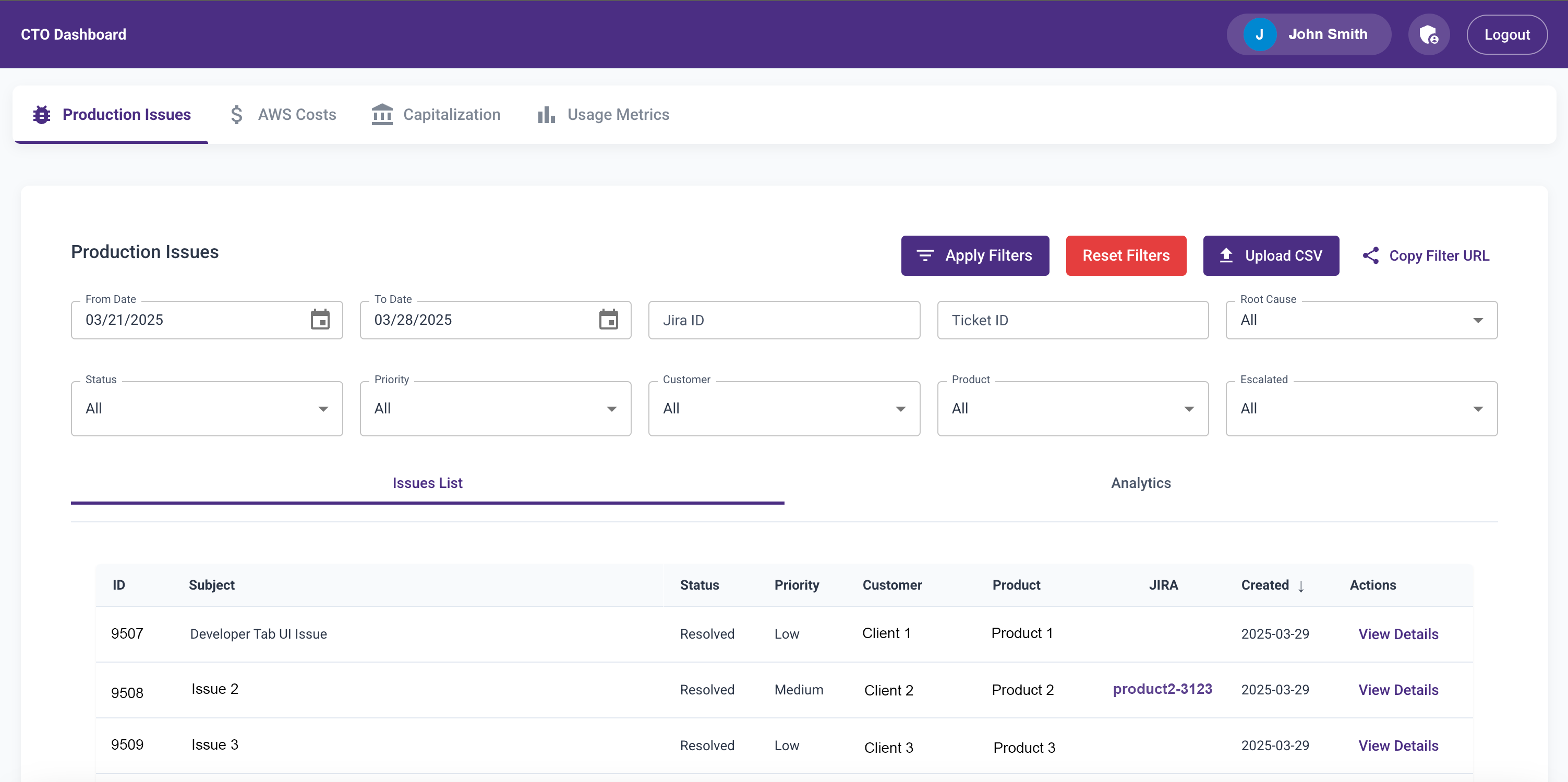
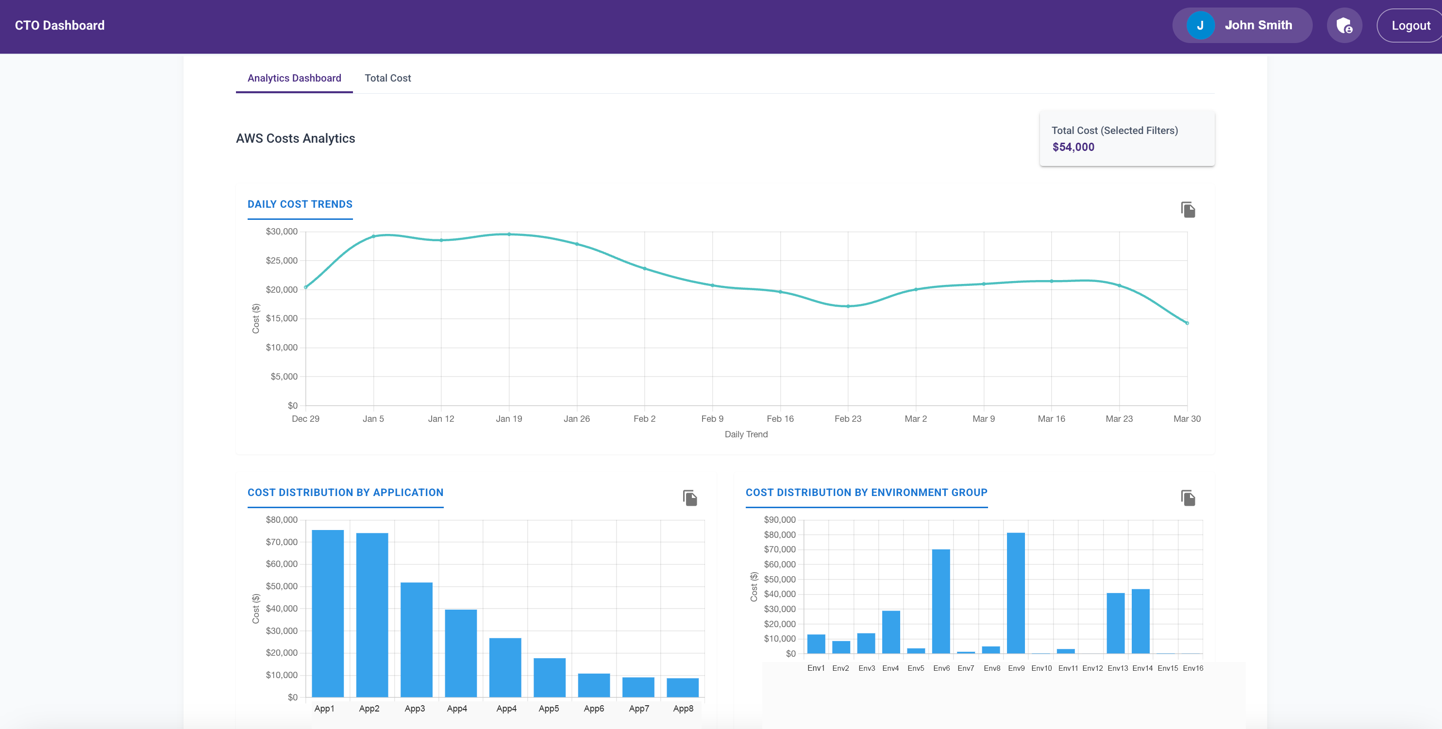
The Build Begins: CTO Dashboard
I decided to build an internal tool I nicknamed CTODashboard—to consolidate everything I needed.
My Tech Stack (via Windsurf):
- Frontend: ReactJS
- Backend: Python (FastAPI)
- Database: Postgres
- Deployment: EC2 (with some help from the SRE team)
I used Windsurf’s Cascade interface to prompt out code, even while attending meetings. It was surprisingly effective… except for one time when a prompt completely messed up my day’s work. Lesson learned: commit code at every working logical step.
In a couple of days, I had:
- A feature to upload the CSV dump
- Filters to slice and dice data
- A paginated data table
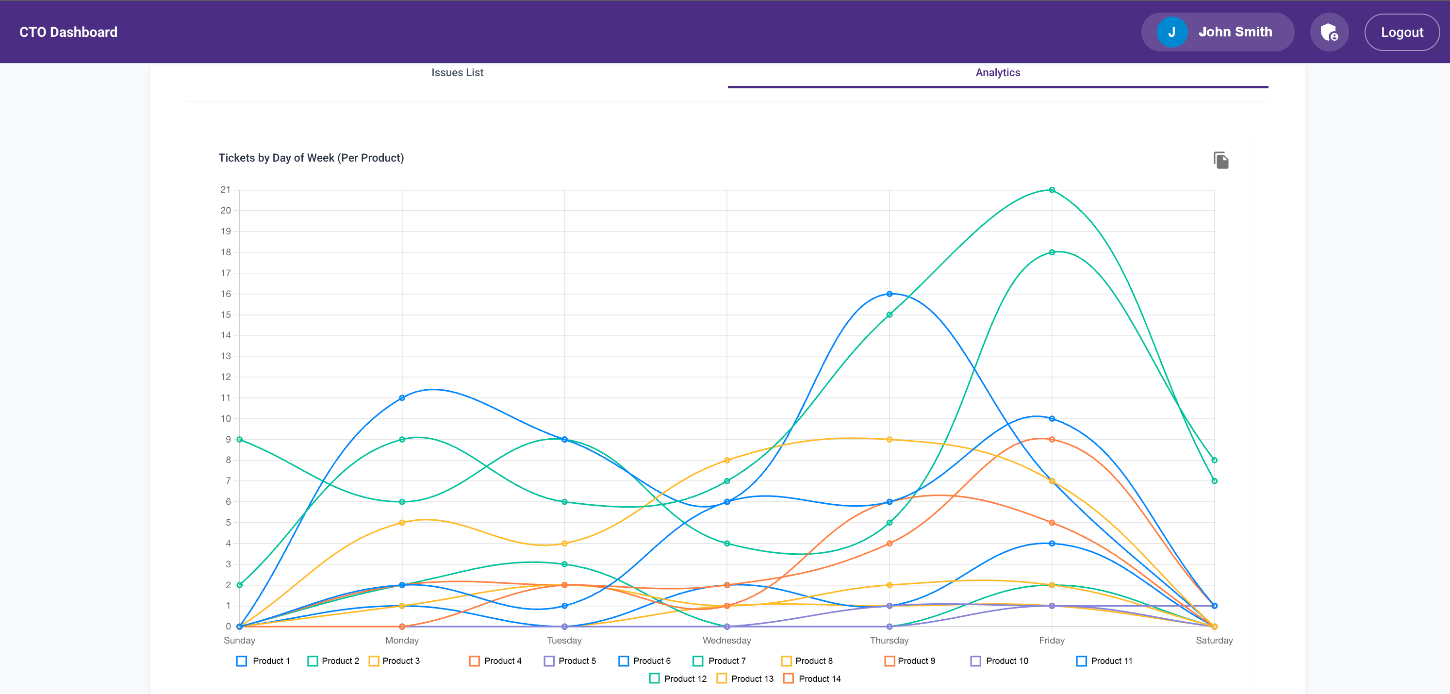
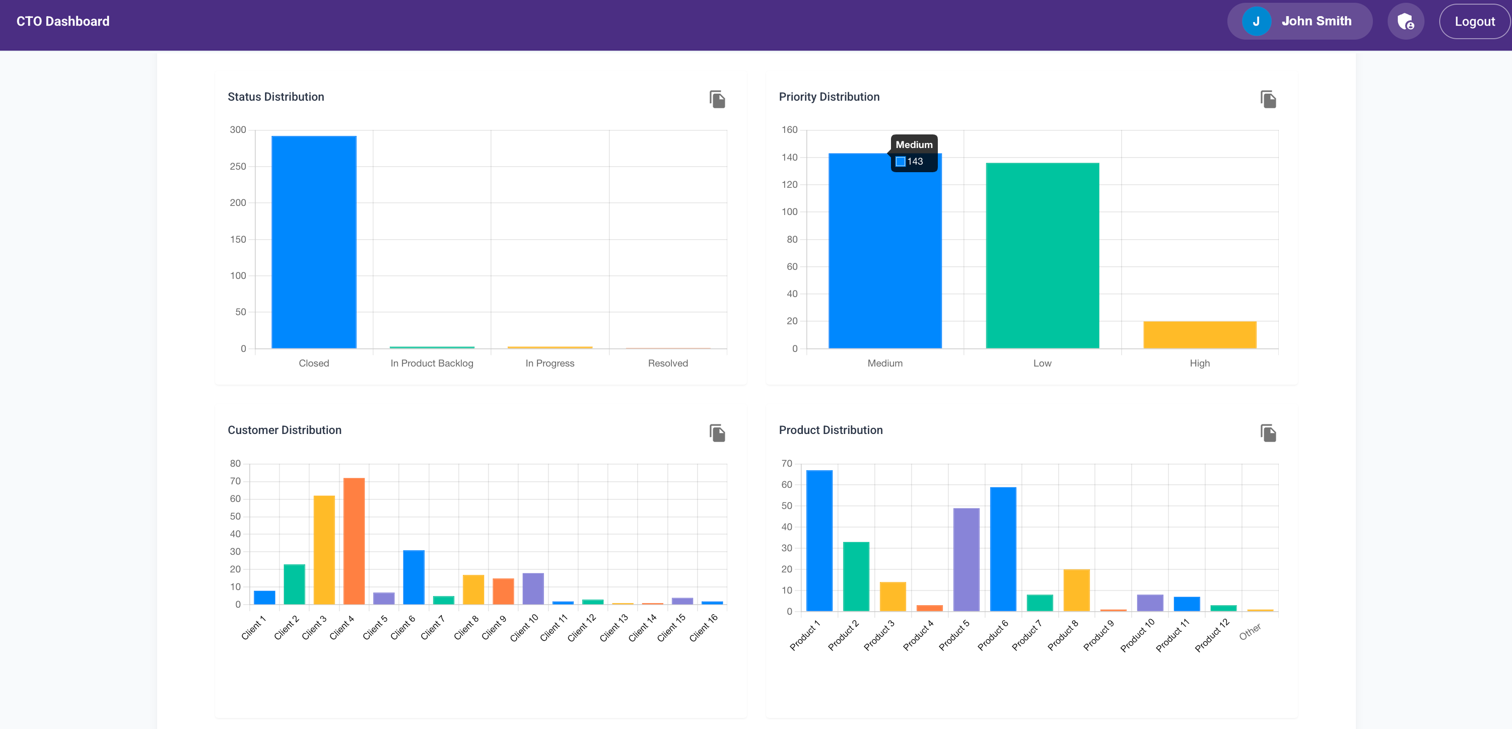
- Trend analytics with visualizations
Even when I hit errors, I just screenshot them or pasted logs into Windsurf and asked it to fix them. It did a decent job. When it hallucinated or got stuck, I just restarted with a fresh Cascade.
I had to rewrite the CSV upload logic manually when the semantic mapping to the backend tables went wrong. But overall, 80% of the code was generated—20% I wrote myself. And I reviewed everything to ensure it worked as intended.
Early Feedback & Iteration
I gave access to a couple of colleagues for early feedback. It was overwhelmingly positive. They even suggested new features like:
- Summarizing long tickets
- Copy-pasting ticket details directly into Slack
- Copying visualizations without taking screenshots
I implemented all of those using Windsurf in just a few more days.
In under a week, I had an MVP that cut my Thursday analysis time from 6+ hours to under 2.
Then Abhay Dandekar, another senior developer, offered to help. He built a Lambda function to call our Helpdesk API every hour to fetch the latest tickets and updates. He got it working in 4 hours—like a boss.
Growing Usage
Word about the dashboard started leaking (okay, I may have leaked it myself 😉). As more people requested access, I had to:
- Add Google Sign-In
- Implement authorization controls
- Build a user admin module
- Secure the backend APIs with proper access control
- Add audit logs to track who was using what
I got all this done over a weekend. It consumed my entire weekend, but it was worth it.
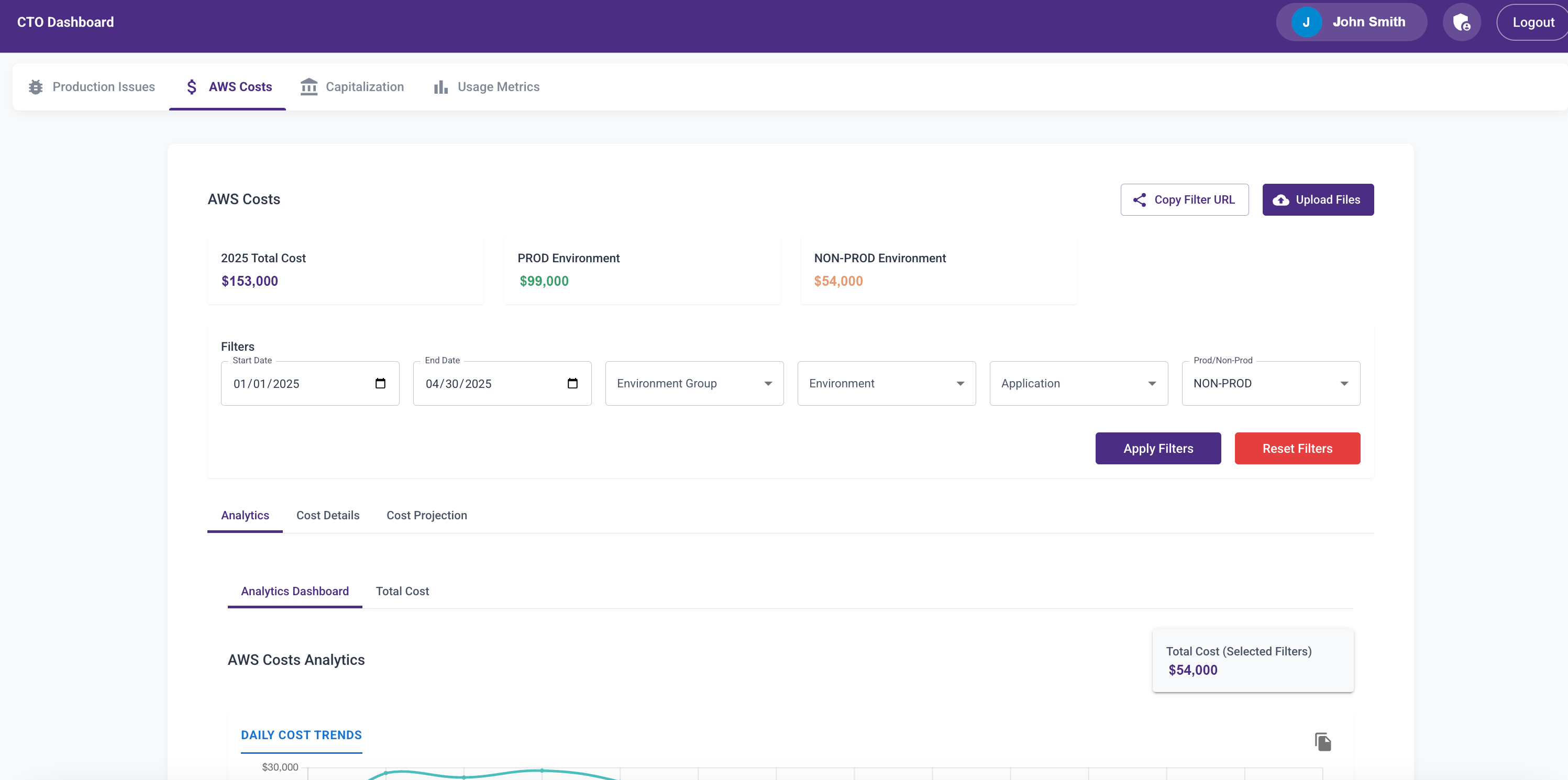
AWS Cost Analytics Module
Next, I added a module to analyze AWS cost trends across production and non-prod environments by product.
Initially, it was another CSV upload feature. Later, Abhay added a Lambda to fetch the data daily. I wanted engineering directors to see the cost implications of design decisions—especially when non-prod environments were always-on.
Before this, I spent 30 minutes daily reviewing AWS cost trends. Once the dashboard launched, engineers started checking it themselves. That awareness led to much smarter decisions and significant cost savings.
I added visualizations for:
- Daily cost trends
- Monthly breakdowns
- Environment-specific views
- Product-level costs
More Modules Coming Soon
I’ve since added:
- Usage metrics
- Capitalization tracking
- (In progress): Performance and engineering metrics
The dashboard now has 200+ users, and I’m releasing access in batches to manage performance.
Lessons Learned from VibeCoding
This was a fun experiment to see how far I could go with GenAI-based development using just prompts.
What I Learned:
- Strong system design fundamentals are essential.
- Windsurf can get stuck in loops—step in and take control.
- Commit frequently. Mandatory.
- You’re also the tester—don’t skip this.
- If the app breaks badly, roll back. Don’t fix bad code.
- GenAI editors are great for senior engineers; less convinced about junior devs.
- Model training cutoffs matter—it affects library choices.
- Write smart prompts with guardrails (e.g., “no files >300 lines”).
- GenAI tools struggle to edit large files (my
app.py hit 5,000 lines; I had to refactor manually).
- Use virtual environments—GenAI often forgets.
- Deployments are tedious—I took help from the SRE team for Jenkins/Terraform setup.
- If you love coding, VibeCoding is addictive.
Gratitude
Special thanks to:
- Bhavani Shankar, Navin Kumaran, Geetha Eswaran, and Sabyasachi Rout for helping with deployment scripts and automation (yes, I bugged them a lot).
- Pravin Kumar, Vikas Kishore, Nandini PS, and Prithviraj Subburamanian for feedback and acting as de facto product managers for dashboard features.
25 Sep 2024
Tokenizers
_Co-authored by Tamil Arasan, Selvakumar Murugan and Malaikannan Sankarasubbu
In Natural Language Processing (NLP), one of the foundational steps is transforming human language into a format that computational models can understand. This is where tokenizers come into play. Tokenizers are specialized tools that break down text into smaller units called tokens, and convert these tokens into numerical data that models can process.
Imagine you have the sentence:
Artificial intelligence is revolutionizing technology.
To a human, this sentence is clear and meaningful. But we do not
understand the whole sentence in one shot(okay may be you did, but I am
sure if I gave you a paragraph or a even better an essay, you will not
be able to understand them in one shot), but we make sense of parts of
it like words and then phrases and understand the whole sentence as a
composition of meanings from its parts. It is just how things work,
regardless whether we are trying to make a machine mimic our language
understanding or not. This has nothing to do with the reason ML models
or even computers in general work with numbers. It is purely how
language works and there is no going around it.
ML models like everything else we run on computers can only work with
numbers, and we need to transform the text into number or series of
numbers (since we have more than one word). We have a lot of freedom
when it comes to how we transform the text into numbers, and as always
with freedom comes complexity. But basically, tokenization as a whole is
a two step process. Finding all the words and assigning a unique
number - an ID to each token.
There are so many ways we can segment a sentence/paragraph into pieces
like phrases, words, sub-words or even individual characters.
Understanding why particular tokenization scheme is better requires a
grasp of how embeddings work. If you're familiar with NLP, you'd ask
"Why? Tokenization comes before the Embedding, right?" Yes, you're
right, but NLP is paradoxical like that. Don't worry we will cover that
as we go.
Background
Before we venture any further, lets understand the difference between
Neural networks and our typical computer programs. We all know by now
that for traditional computer programs, we write/translate the rules
into code by hand whereas, NNs learn the rules(mapping across input and
output) from data by the process called training. You see unlike in
normal programming style, where we have a plethora of data-structures
that can help with storing information in any shape or form we want,
along with algorithms that jump up and down, back and forth in a set of
instructions we call code, Neural Networks do not allow us to have all
sorts of control flow we'd like. In Neural Networks, there is only one
direction the "program" can run, left to right.
Unlike in traditional programs where the we can feed a program with
input in complicated ways, in Neural Networks, there are only fixed
number of ways, we can feed and it is usually in the form of vectors
(fancy name for list of numbers) and the vectors are of fixed size (or
dimension more precisely). In most DNNs, input and output sizes are
fixed regardless of the problem it is trying to solve. For example, CNNs
the input (usually image) size and number of channels is fixed. In RNNs,
the embedding dimensions, input vocabulary size, number of output labels
(classification problem e.g: sentiment classification) and or output
vocabulary size (text generation problems e.g: QA, translation) are all
fixed. In Transformer networks even the sentence length is fixed. This
is not a bad thing, constraints like these enable the network to
compress and capture the necessary information.
Also note that there are only few tools to test "equality" or
"relevance" or "correctness" for things inside the network because
only things that dwell inside the network are vectors. Cosine similarity
and attention scores are popular. You can think of vectors as variables
that keep track of state inside neural network program. But unlike in
traditional programs where you can declare variables as you'd like and
print them for troubleshooting, in networks the vector-variables are
only meaningful only at the boundaries of the layers(not entirely true)
within the networks.
Lets take a look at the simplest example to understand why just pulling
a vector from anywhere in the network will not be of any value for us.
In the following code, three functions perform the identical calculation
despite their code is slightly different. The unnecessarily
intentionally named variables temp and growth_factor need not be
created as exemplified by the first function, which directly embodies
the compound interest calculation formula, $A = P(1+\frac{R}{100})^{T}$.
When compared to temp, the variable growth_factor hold a more
meaningful interpretation - represents how much the money will grow due
to compounding interest over time. For more complicated formulae and
functions, we might create intermediate variables so that the code goes
easy on the eye, but they have no significance to the operation of the
function.
def compound_interest_1(P,R,T):
    A = P * (math.pow((1 + (R/100)),T))
    CI = A - P
    return CI

def compound_interest_2(P,R,T):
    temp = (1 + (R/100))
    A = P * (math.pow(temp, T))
    CI = A - P
    return CI

def compound_interest_3(P,R,T):
    growth_factor = (math.pow((1 + (R/100)),T))
    A = P * growth_factor
    CI = A - P
    return CI
Another example to illustrate from operations perspective. Clock
arithmetic. Lets assign numbers 0 through 7 to weekdays starting from
Sunday to Saturday.
Table 1
| Sun |
Mon |
Tue |
Wed |
Thu |
Fri |
Sat |
| 0 |
1 |
2 |
3 |
4 |
5 |
6 |
John Conway suggests, a mnemonic device for thinking of the days of
the week as Noneday, Oneday, Twosday, Treblesday, Foursday, Fiveday,
and Six-a-day.
So if you want to know what day it is 137 days from today if today is
say, Thursday (i.e. 4). We can do $(4+137) mod 7 => 1$ i.e Monday. As
you can see adding numbers(days) in clock arithmetic results in a
meaningful output. You can days together to get another day. Okay lets
ask the question can we multiply two days together? Is it is in anyway
meaningful to multiply days? Just because we can multiply any number
mathematically, is it useful to do so in our clock arithmetic?
All of this digression is to emphasize that the embedding is deemed
to capture the meaning of words, vector from the last layers is deemed
to capture the meaning of a sentence lets say. But when you take a
vector (just because you can) within the layers for instance, it does
not refer to any meaningful unit such as words or phrases and sentence
as we understand it.
A little bit of history
If you're old enough, you might remember that before transformers
became standard paradigm in NLP, we had another one EEAP (Embed, Encode,
Attend, Predict). I am grossly oversimplifying here, but you can think
of it as follows,
- Embedding
-
Captures the meaning of words A matrix of size $N \times D$, where
- $N$ is the size of the vocabulary, i.e unique number of words in
the language
- $D$ is the dimension of embedding, vector corresponding to each
word.
Lookup the word-vector (embedding) for each word
- Encoding
- Find the meaning of a sentence, by using the meaning captured in
embeddings of the constituent words with help of RNNs like LSTM, GRU
or transformers like BERT, GPT that take the embeddings and produce
vector(s) for whole the sequence.
- Prediction
- Depending upon the task at hand, either assigns a label to the input
sentence, or generate another sentence word by word.
- Attention
- Helps with Prediction by focusing on what is important right now by
drawing a probability distribution (normalized attention scores)
over the all words. Words with high score are deemed important.
As you can see above, $N$ is the vocabulary size, i.e unique number of
words in the language. And handful of years ago, language usually meant
the corpus at hand (in order of few thousands of sentences) and datasets
like CNN/DailyMail were considered huge. There were clever tricks like
anonymizing named entities to force the ML models to focus on language
specific features like grammar instead of open world words like names of
Places, Presidents, Corporations and Countries, etc. Good times they
were! Point is, it is possible that the corpus you have in your
possession might not have all the words of the language. As we have
seen, the size of the Embedding must be fixed before training the
network. By good fortune if you stumble upon a new dataset and hence new
words, adding them to your model was not easy, because Embedding needs
to extend to accommodate this new (OOV) words and that requires
retraining of the whole network. OOV means Out Of the current model's
Vocabulary. And this is why simply segmenting the text on empty spaces
will not work.
With that background, lets dive in.
Tokenization
Tokenization is the process of segmenting the text into individual
pieces (usually words) so that ML model can digest them. It is the very
first step in any NLP system and influences everything that follows. For
understanding impact of tokenization, we need to understand how
embeddings and sentence length influence the model. We will call
sentence length as sequence length from here on, because sentence is
understood to be sequence of words, and we will experiment with sequence
of different things not just words, which we will call tokens.
Tokens can be anything
- Words -
"telephone" "booth" "is" "nearby" "the" "post" "office"
- Multiword Expressions (MWEs) -
"telephone booth" "is" "nearby" "the" "post office"
- Sub-words -
"tele" "#phone" "booth" "is" "near " "#by" "the" "post" "office"
- Characters -
"t" "e" "l" "e" "p" ... "c" "e"
We know segmenting the text based on empty spaces will not work, because
the vocabulary will keep growing. What about punctuations? Surely they
will help with words
don't, won't, aren't, o'clock, Wendy's, co-operation{.verbatim} etc,
same reasoning applies here too. Moreover segmenting at punctuations
will create different problems, e.g: I.S.R.O > I, S, R, O{.verbatim}
which is not ideal.
Objectives of Tokenization
The primary objectives of tokenization are:
- Handling OOV
- Tokenizers should be able to segment the text into pieces so that
any word in the language whether it is in the dataset or not, any
word we might conjure in foreseeable future, whether it is a
technical/domain specific terminology that scientists might utter to
sound intelligent or commonly used by everyone in day to day life.
An ideal tokenizer should be able to deal with all and any of them.
- Efficiency
- Reducing the size (length) of the input text to make computation
feasible and faster.
- Meaningful Representation
- Capturing the semantic essence of the text so that the model can
learn effectively. Which we will discuss a bit later.
Simple Tokenization Methods
Go through the code below, and see if you can make any inferences on the
table produced. It reads the book The
Republic and
counts the tokens on character, word and sentence levels and also
indicated the number of unique tokens in the whole book.
Code
``` {.python results=”output raw” exports=”both”}
from collections import Counter
from nltk.tokenize import sent_tokenize
with open(‘plato.txt’) as f:
text = f.read()
words = text.split()
sentences = sent_tokenize(text)
char_counter = Counter()
word_counter = Counter()
sent_counter = Counter()
char_counter.update(text)
word_counter.update(words)
sent_counter.update(sentences)
print(‘#+name: Vocabulary Size’)
print(‘|Type|Vocabulary Size|Sequence Length|’)
print(f’|Unique Characters|{len(char_counter)}|{len(text)}’)
print(f’|Unique Words|{len(word_counter)}|{len(words)}’)
print(f’|Unique Sentences|{len(sent_counter)}|{len(sentences)}’)
**Table 2**

| Type              | Vocabulary Size | Sequence Length |
| ----------------- | --------------- | --------------- |
| Unique Characters | 115             | 1,213,712       |
| Unique Words      | 20,710          | 219,318         |
| Unique Sentences  | 7,777           | 8,714           |


## Study

Character-Level Tokenization

:   In this most elementary method, text is broken down into individual
    characters.

    *\"data\"* \> `"d" "a" "t" "a"`{.verbatim}

Word-Level Tokenization

:   This is the simplest and most used (before sub-word methods became
    popular) method of tokenization, where text is split into individual
    words based on spaces and punctuation. Still useful in some
    applications and as a pedagogical launch pad into other tokenization
    techniques.

    *\"Machine learning models require data.\"* \>
    `"Machine", "learning", "models", "require", "data", "."`{.verbatim}

Sentence-Level Tokenization

:   This approach segments text into sentences, which is useful for
    tasks like machine translation or text summarization. Sentence
    tokenization is not as popular as we\'d like it to be.

    *\"Tokenizers convert text. They are essential in NLP.\"* \>
    `"Tokenizers convert text.", "They are essential in NLP."`{.verbatim}

n-gram Tokenization

:   Instead of using sentences as a tokens, what if you could use
    phrases of fixed length. The following shows the n-grams for n=2,
    i.e 2-gram or bigram. Yes the `n`{.verbatim} in the n-grams stands
    for how many words are chosen. n-grams can also be built from
    characters instead of words, though not as useful as word level
    n-grams.

    *\"Data science is fun\"* \>
    `"Data science", "science is", "is fun"`{.verbatim}.


**Table 3**

| Tokenization | Advantages                             | Disadvantages                                        |
| ------------ | -------------------------------------- | ---------------------------------------------------- |
| Character    | Minimal vocabulary size                | Very long token sequences                            |
|              | Handles any possible input             | Require huge amount of compute                       |
| Word         | Easy to implement and understand       | Large vocabulary size                                |
|              | Preserves meaning of words             | Cannot cover the whole language                      |
| Sentence     | Preserves the context within sentences | Less granular; may miss important word-level details |
|              | Sentence-level semantics               | Sentence boundary detection is challenging           |

As you can see from the table, the vocabulary size and sequence length
have inverse correlation. The Neural networks requires that the tokens
should be present in many places and many times. That is how the
networks understand words. Remember when you don\'t know the meaning of
a word, you ask someone to use it in sentences? Same thing here, the
more sentences the token is present, the better the network can
understand it. But in case of sentence tokenization, you can see there
are as many tokens in its vocabulary as in the tokenized corpus. It is
safe to say that each token is occuring only once and that is not a
healthy diet for a network. This problem occurs in word-level
tokenization too but it is subtle, the out-of-vocabulary(OoV) problem.
To deal with OOV we need to stay between character level and word-level
tokens, enter \>\>\> sub-words \<\<\<.

# Advanced Tokenization Methods

Subword tokenization is an advanced tokenization technique that breaks
text into smaller units, smaller than words. It helps in handling rare
or unseen words by decomposing them into known subword units. Our hope
is that, the sub-words decomposed from text, can be used to compose new
unseen words and so act as the tokens for the unseen words. Common
algorithms include Byte Pair Encoding (BPE), WordPiece, SentencePiece.

*\"unhappiness\"* \> `"un", "happi", "ness"`{.verbatim}

BPE is originally a technique for compression of data. Repurposed to
compress text corpus by merging frequently occurring pairs of characters
or subwords. Think of it like what and how little number of unique
tokens you need to recreate the whole book when you are free to arrange
those tokens in a line as many time as you want.

Algorithm

:   1.  *Initialization*: Start with a list of characters (initial
        vocabulary) from the text(whole corpus).
    2.  *Frequency Counting*: Count all pair occurrences of consecutive
        characters/subwords.
    3.  *Pair Merging*: Find the most frequent pair and merge it into a
        single new subword.
    4.  *Update Text*: Replace all occurrences of the pair in the text
        with the new subword.
    5.  *Repeat*: Continue the process until reaching the desired
        vocabulary size or merging no longer provides significant
        compression.

Advantages

:   -   Reduces the vocabulary size significantly.
    -   Handles rare and complex words effectively.
    -   Balances between word-level and character-level tokenization.

Disadvantages

:   -   Tokens may not be meaningful standalone units.
    -   Slightly more complex to implement.

## Trained Tokenizers

WordPiece and SentencePiece tokenization methods are extensions of BPE
where the vocabulary is not merely created by assuming merging most
frequent pair. These variants evaluate whether the given merges were
useful or not by measuring how much each merge maximizes the likelihood
of the corpus. In simple words, lets take two vocabularies, before and
after the merges, and train two language models and the model trained on
vocabulary after the merges have lower perplexity(think loss) then we
assume that the merges were useful. And we need to repeat this every
time we make a merge. Not practical, and hence there some mathematical
tricks we use to make this more practical that we will discuss in a
future post.

The iterative merging process is the training of tokenizer and this
training is different training of actual models. There are python
libraries for training your own tokenizer, but when you\'re planning to
use a pretrained language model, it is better to stick with the
pretrained tokenizer associated with that model. In the following
section we see how to train a simple BPE tokenizer, SentencePiece
tokenizer and how to use BERT tokenizer that comes with huggingface\'s
`transformers`{.verbatim} library.

## Tokenization Techniques Used in Popular Language Models

### Byte Pair Encoding (BPE) in GPT Models

GPT models, such as GPT-2 and GPT-3, utilize Byte Pair Encoding (BPE)
for tokenization.

``` {.python results="output code" exports="both"}
from tokenizers import Tokenizer
from tokenizers.models import BPE
from tokenizers.trainers import BpeTrainer
from tokenizers.pre_tokenizers import Whitespace

tokenizer =  Tokenizer(BPE(unk_token="[UNK]"))
tokenizer.pre_tokenizer = Whitespace()
trainer = BpeTrainer(special_tokens=["[UNK]", "[CLS]", "[SEP]", "[PAD]", "[MASK]"],
                     vocab_size=30000)
files = ["plato.txt"]

tokenizer.train(files, trainer)
tokenizer.model.save('.', 'bpe_tokenizer')

output = tokenizer.encode("Tokenization is essential first step for any NLP model.")
print("Tokens:", output.tokens)
print("Token IDs:", output.ids)
print("Length: ", len(output.ids))
Tokens: ['T', 'oken', 'ization', 'is', 'essential', 'first', 'step', 'for', 'any', 'N', 'L', 'P', 'model', '.']
Token IDs: [50, 6436, 2897, 127, 3532, 399, 1697, 184, 256, 44, 42, 46, 3017, 15]
Length:  14
SentencePiece in T5
T5 models use a Unigram Language Model for tokenization, implemented via
the SentencePiece library. This approach treats tokenization as a
probabilistic model over all possible tokenizations.
import sentencepiece as spm
spm.SentencePieceTrainer.Train('--input=plato.txt --model_prefix=unigram_tokenizer --vocab_size=3000 --model_type=unigram')
``` {.python results=”output code” exports=”both”}
import sentencepiece as spm
sp = spm.SentencePieceProcessor()
sp.Load(“unigram_tokenizer.model”)
text = “Tokenization is essential first step for any NLP model.”
pieces = sp.EncodeAsPieces(text)
ids = sp.EncodeAsIds(text)
print(“Pieces:”, pieces)
print(“Piece IDs:”, ids)
print(“Length: “, len(ids))
``` python
Pieces: ['▁To', 'k', 'en', 'iz', 'ation', '▁is', '▁essential', '▁first', '▁step', '▁for', '▁any', '▁', 'N', 'L', 'P', '▁model', '.']
Piece IDs: [436, 191, 128, 931, 141, 11, 1945, 123, 962, 39, 65, 17, 499, 1054, 1441, 1925, 8]
Length:  17
WordPiece Tokenization in BERT
``` {.python results=”output code”}
from transformers import BertTokenizer
tokenizer = BertTokenizer.from_pretrained(‘bert-base-uncased’)
text = “Tokenization is essential first step for any NLP model.”
encoded_input = tokenizer(text, return_tensors=’pt’)
print(“Tokens:”, tokenizer.convert_ids_to_tokens(encoded_input[‘input_ids’][0]))
print(“Token IDs:”, encoded_input[‘input_ids’][0].tolist())
print(“Length: “, len(encoded_input[‘input_ids’][0].tolist()))
```
Summary of Tokenization Methods
Table 4
| Method |
Length |
Tokens |
| BPE |
14 |
[‘T’, ‘oken’, ‘ization’, ‘is’, ‘essential’, ‘first’, ‘step’, ‘for’, ‘any’, ‘N’, ‘L’, ‘P’, ‘model’, ‘.’] |
| SentencePiece |
17 |
[‘▁To’, ‘k’, ‘en’, ‘iz’, ‘ation’, ‘▁is’, ‘▁essential’, ‘▁first’, ‘▁step’, ‘▁for’, ‘▁any’, ‘▁’, ‘N’, ‘L’, ‘P’, ‘▁model’, ‘.’] |
| WordPiece (BERT) |
12 |
[‘token’, ‘##ization’, ‘is’, ‘essential’, ‘first’, ‘step’, ‘for’, ‘any’, ‘nl’, ‘##p’, ‘model’, ‘.’] |
Different tokenization methods give different results for the same input
sentence. As we add more data to the tokenizer training, the differences
between WordPiece and SentencePiece might decrease, but they will not
vanish, because of the difference in their training process.
Table 5
| Model |
Tokenization Method |
Library |
Key Features |
| GPT |
Byte Pair Encoding |
tokenizers |
Balances vocabulary size and granularity |
| BERT |
WordPiece |
transformers |
Efficient vocabulary, handles morphology |
| T5 |
Unigram Language Model |
sentencepiece |
Probabilistic, flexible across languages |
Tokenization and Non English Languages
Tokenizing text is complex, especially when dealing with diverse
languages and scripts. Various challenges can impact the effectiveness
of tokenization.
Tokenization Issues with Complex Languages: With a focus on Tamil
Tokenizing text in languages like Tamil presents unique challenges due
to their linguistic and script characteristics. Understanding these
challenges is essential for developing effective NLP applications that
handle Tamil text accurately.
Challenges in Tokenizing Tamil Language
-
1. Agglutinative Morphology
Tamil is an agglutinative language, meaning it forms words by
concatenating morphemes (roots, suffixes, prefixes) to convey
grammatical relationships and meanings. A single word may express
what would be a full sentence in English.
- Impact on Tokenization
-
- Words can be very lengthy and contain many morphemes.
- போகமுடியாதவர்களுக்காவேயேதான்
-
2. Punarchi and Phonology
Tamil specific rules on how two words can be combined and resulting
word may not be phonologically identical to its parts. The
phonological transformations can cause problems with TTS/STT systems
too.
- Impact on Tokenization
-
- Surface forms of words may change when combined, making
boundary detection challenging.
- மரம் + வேர் > மரவேர்
- தமிழ் + இனிது > தமிழினிது
-
3. Complex Script and Orthography
Tamil alphabet representation in Unicode is suboptimal for
everything except for standardized storage format. Even simple
operations that are intuitive for native Tamil speaker, are harder
to implement because of this. Techniques like BPE applied on Tamil
text will break words at completely inappropriate points like
cutting an uyirmei letter into consonant and diacritic resulting in
meaningless output.
தமிழ் > த ம ி ழ, ்
Strategies for Effective Tokenization of Tamil Text
-
Language-Specific Tokenizers
Train Tamil specific subword tokenizers with initial seed tokens
prepared by better preprocessing techniques to avoid
[problem-3]{.spurious-link
target=”*3. Complex Script and Orthography”} type cases. Use
morphological analyzers to decompose words into root and affixes,
aiding in understanding and processing complex word forms.
Choosing the Right Tokenization Method
Challenges in Tokenization
- Ambiguity: Words can have multiple meanings, and tokenizers cannot
capture context. Example: The word "lead" can be a verb or a
noun.
- Handling Special Characters and Emojis: Modern text often includes
emojis, URLs, and hashtags, which require specialized handling.
- Multilingual Texts: Tokenizing text that includes multiple languages
or scripts adds complexity, necessitating adaptable tokenization
strategies.
Best Practices for Effective Tokenization
- Understand Your Data: Analyze the text data to choose the most
suitable tokenization method.
- Consider the Task Requirements: Different NLP tasks may benefit from
different tokenization granularities.
- Use Pre-trained Tokenizers When Possible: Leveraging existing
tokenizers associated with pre-trained models can save time and
improve performance.
- Normalize Text Before Tokenization: Cleaning and standardizing text
31 Aug 2024
Vector Databases 101
_Co-authored by Angu S KrishnaKumar, Kamal raj Kanagarajan and Malaikannan Sankarasubbu
Introduction
In the world of Large Language Models (LLMs), vector databases play a pivotal role in Retrieval Augmented Generation (RAG) applications.** These specialized databases are designed to store and retrieve high-dimensional vectors, which represent complex data structures like text, images, and audio. By leveraging vector databases, LLMs can access vast amounts of information and generate more informative and accurate responses. Retrieval Augmented Generation (RAG) is a technique that combines the power of large language models (LLMs) with external knowledge bases to generate more informative and accurate responses. By retrieving relevant information from a knowledge base and incorporating it into the LLM’s generation process, RAG can produce more comprehensive and contextually appropriate outputs.
How RAG Works:
- User Query: A user submits a query or prompt to the RAG system.
- Information Retrieval: The system retrieves relevant information from a knowledge base based on the query. VectorDBs play a key role in this. Embeddings aka vectors are stored in VectorDB and retrieval is done using similarity measures.
- Language Model Generation: The retrieved information is fed into a language model, which generates a response based on the query and the retrieved context.
In this blog series, we will delve into the intricacies of vector databases, exploring their underlying principles, key features, and real-world applications. We will also discuss the advantages they offer over traditional databases and how they are transforming the way we store, manage, and retrieve data.
What is a Vector?
A vector is a sequence of numbers that forms a group. For example
- (3) is a one dimensional vector.
- (2,8) is a two dimensional vector.
- (12,6,7,4) is a four dimensional vector.
A vector can be represented as by plotting on a graph. Lets take a 2D example
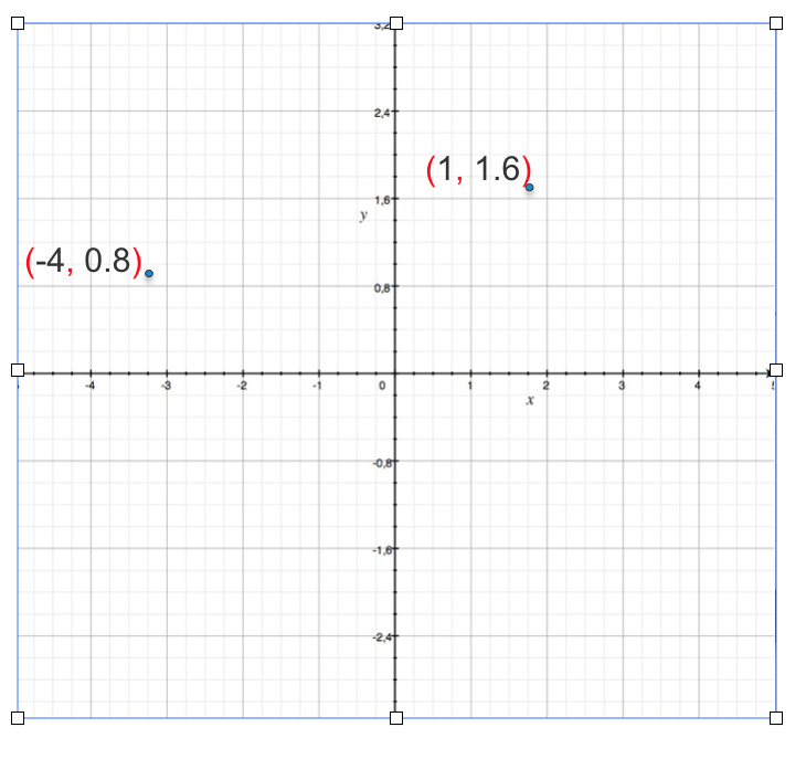
We can only visualize 3 dimensions, anything more than that you can just say it not visualize.
Below is an example of 4 dimension vector representation of the word king
What is a Vector Database?
A Vector Database (VectorDB) is a specialized database system designed to store, manage, and efficiently query high-dimensional vector data. Unlike traditional relational databases that work with structured data in tables, VectorDBs are optimized for handling vector embeddings – numerical representations of data in multi-dimensional space.
In a VectorDB:
- Each item (like a document, image, or concept) is represented as a vector – a list of numbers that describe the item’s features or characteristics.
- These vectors are stored in a way that allows for fast similarity searches and comparisons.
- The database is optimized for operations like finding the nearest neighbors to a given vector, which is crucial for many AI and machine learning applications.
VectorDBs are particularly useful in scenarios where you need to find similarities or relationships between large amounts of complex data, such as in recommendation systems, image recognition, or natural language processing tasks.
Key Concepts
-
Vector Embeddings
- Vector embeddings are numerical representations of data in a multi-dimensional space.
- They capture semantic meaning and relationships between different pieces of information.
- In natural language processing, word embeddings are a common type of vector embedding. Each word is represented by a vector of real numbers, where words with similar meanings are closer in the vector space.
- For detail concepts of embedding please refer to earlier blog Embeddings
Let’s look at an example of Word Vector output generated by Word2Vec
from gensim.models import Word2Vec

# Example corpus (a list of sentences, where each sentence is a list of words)
sentences = [
    ["machine", "learning", "is", "fascinating"],
    ["gensim", "is", "a", "useful", "library", "for", "word", "embeddings"],
    ["vector", "representations", "are", "important", "for", "NLP", "tasks"]
]

# Train a Word2Vec model with 300-dimensional vectors
model = Word2Vec(sentences, vector_size=300, window=5, min_count=1, workers=4)

# Get the 300-dimensional vector for a specific word
word_vector = model.wv['machine']

# Print the vector
print(f"Vector for 'machine': {word_vector}")
Sample Output for 300 dimension vector
Vector for 'machine': [ 2.41737941e-03 -1.42750892e-03 -4.85344668e-03  3.12493594e-03, 4.84531874e-03 -1.00165956e-03  3.41092921e-03 -3.41384278e-03, 4.22888929e-03  1.44586214e-03 -1.35438916e-03 -3.27448458e-03
  4.70721726e-03 -4.50850562e-03  2.64214014e-03 -3.29884756e-03, -3.13906092e-03  1.09677911e-03 -4.94637461e-03  3.32896863e-03,2.03538216e-03 -1.52456785e-03  2.28793684e-03 -1.43519988e-03, 4.34566711e-03 -1.94705374e-03  1.93231280e-03  4.34081139e-03
  ...
  3.40303702e-03  1.58637420e-03 -3.31261402e-03  2.01543484e-03,4.39879852e-03  2.54576413e-03 -3.30528596e-03  3.01509819e-03,2.15555660e-03  1.64605413e-03  3.02376228e-03 -2.62048110e-03
  3.80181967e-03 -3.14147812e-03  2.23554621e-03  2.68812295e-03,1.80951719e-03  1.74256027e-03 -2.47024545e-03  4.06702763e-03,2.30203426e-03 -4.75471295e-03 -3.66776927e-03  2.06539119e-03]
- High Dimensional Space
- Vector databases typically work with vectors that have hundreds or thousands of dimensions. This high dimensionality allows for rich and nuanced representations of data.
- For example:
- A word might be represented by 300 dimensions
- An image could be represented by 1000 dimensions
- A user’s preferences might be captured in 500 dimensions
Why do you need a Vector Database when there is RDBMS like PostGreSQL or NoSQL DB like Elastic Search or MongoDB?
RDBMS
RDBMS are designed to store and manage structured data in a tabular format. They are based on the relational model, which defines data as a collection of tables, where each table represents a relation.
Key components of RDBMS:
- Tables: A collection of rows and columns, where each row represents a record and each column represents an attribute.
- Rows: Also known as records, they represent instances of an entity.
- Columns: Also known as attributes, they define the properties of an entity.
- Primary key: A unique identifier for each row in a table.
- Foreign key: A column in one table that references the primary key of another table, establishing a relationship between the two tables.
- Normalization: A process of organizing data into tables to minimize redundancy and improve data integrity.
Why RDBMS don’t apply to storing vectors:
- Data Representation:
- RDBMS store data in a tabular format, where each row represents an instance of an entity and each column represents an attribute.
- Vectors are represented as a sequence of numbers, which doesn’t fit well into the tabular structure of RDBMS.
- Query Patterns:
- RDBMS are optimized for queries based on joining tables and filtering data based on specific conditions.
- Vector databases are optimized for similarity search, which involves finding vectors that are closest to a given query vector. This type of query doesn’t align well with the traditional join-based queries of RDBMS.
- Data Relationships:
- RDBMS define relationships between entities using foreign keys and primary keys.
- In vector databases, relationships are implicitly defined by the proximity of vectors in the vector space. There’s no explicit need for foreign keys or primary keys.
- Performance Considerations:
- RDBMS are often optimized for join operations and range queries.
- Vector databases are optimized for similarity search, which requires efficient indexing and partitioning techniques.
Let’s also look at a table for a comparison of features
| Feature |
VectorDB |
RDBMS |
| Dimensional Efficiency |
Designed to handle high-dimensional data efficiently |
Performance degrades rapidly as dimensions increase |
| Similarity Search |
Implement specialized algorithms for fast approximate nearest neighbor (ANN) searches |
Lack native support for ANN algorithms, making similarity searches slow and computationally expensive |
| Indexing for Vector Spaces |
Use index structures optimized for vector data (e.g., HNSW, IVF) |
Rely on B-trees and hash indexes, which become ineffective in high-dimensional spaces |
| Vector Operations |
Provide built-in, optimized support for vector operations |
Require complex, often inefficient SQL queries to perform vector computations |
| Scalability for Vector Data |
Designed to distribute vector data and parallelize similarity searches across multiple nodes efficiently |
While scalable for traditional data, they’re not optimized for distributing and querying vector data at scale |
| Real-time Processing |
Optimized for fast insertions and queries of vector data, supporting real-time applications |
May struggle with the speed requirements of real-time vector processing, especially at scale |
| Storage Efficiency |
Use compact, specialized formats for storing dense vector data |
Less efficient when storing high-dimensional vectors, often requiring more space and slower retrieval |
| Machine Learning Integration |
Seamlessly integrate with ML workflows, supporting operations common in AI applications |
Require additional processing and transformations to work effectively with ML pipelines |
| Approximate Query Support |
Often support approximate queries, trading off some accuracy for significant speed improvements |
Primarily designed for exact queries, lacking native support for approximate vector searches |
In a nutshell, RDBMS are well-suited for storing and managing structured data, but they are not optimized for storing and querying vectors. Vector databases, on the other hand, are specifically designed for handling vectors and performing similarity search operations.
NoSQL Databases
NoSQL databases are designed to handle large datasets and unstructured or semi-structured data that don’t fit well into the relational model. They offer flexibility in data structures, scalability, and high performance.
Common types of NoSQL databases include:
- Key-value stores: Store data as key-value pairs.
- Document stores: Store data as documents, often in JSON or BSON format.
- Wide-column stores: Store data in wide columns, where each column can have multiple values.
- Graph databases: Store data as nodes and relationships, representing connected data.
Key characteristics of NoSQL databases:
- Flexibility: NoSQL databases offer flexibility in data structures, allowing for dynamic schema changes and accommodating evolving data requirements.
- Scalability: Many NoSQL databases are designed to scale horizontally, allowing for better performance and scalability as data volumes grow.
- High performance: NoSQL databases often provide high performance, especially for certain types of workloads.
- Eventual consistency: Some NoSQL databases prioritize availability and performance over strong consistency, offering eventual consistency guarantees.
Why NoSQL Databases Might Not Be Ideal for Storing and Retrieving Vectors
While NoSQL databases offer many advantages, they might not be the best choice for storing and retrieving vectors due to the following reasons:
- Data Representation: NoSQL databases, while flexible, might not be specifically optimized for storing and querying high-dimensional vectors. The data structures used in NoSQL databases might not be the most efficient for vector-based operations.
- Query Patterns: NoSQL databases are often designed for different query patterns than vector-based operations. While they can handle complex queries, they might not be as efficient for similarity search, which is a core operation for vector databases.
- Performance Considerations:
- Indexing: NoSQL databases often use different indexing techniques than RDBMS. While they can be efficient for certain types of queries, they might not be as optimized for vector-based similarity search.
- Memory requirements: For vector-based operations, especially in large-scale applications, the memory requirements can be significant. NoSQL databases like Elasticsearch, which are often used for full-text search and analytics, might require substantial memory resources to handle large vector datasets efficiently.
Elasticsearch as an Example:
Elasticsearch is a popular NoSQL database often used for full-text search and analytics. While it can be used to store and retrieve vectors, there are some considerations:
- Memory requirements: Storing and indexing large vector datasets in Elasticsearch can be memory-intensive, especially for high-dimensional vectors.
- Query performance: The performance of vector-based queries in Elasticsearch can depend on factors like the number of dimensions, the size of the dataset, and the indexing strategy used.
- Specialized plugins: Elasticsearch offers plugins like the
knn plugin that can be used to optimize vector-based similarity search. However, these plugins might have additional performance and memory implications.
In a nutshell, while NoSQL databases offer many advantages, their suitability for storing and retrieving vectors depends on specific use cases and requirements. For applications that heavily rely on vector-based similarity search and require high performance, specialized vector databases might be a more appropriate choice.
A Deeper Dive into Similarity Search in Vector Databases
Similarity search is a fundamental operation in vector databases, involving finding the closest matches to a given query vector from a large dataset of vectors. This is crucial for applications like recommendation systems, image search, and natural language processing.
Similarity measures, algorithms, and data structures are crucial for efficient similarity search. Similarity measures (e.g., cosine, Euclidean) quantify the closeness between vectors. Algorithms (e.g., brute force, LSH, HNSW) determine how vectors are compared and retrieved. Data structures (e.g., inverted indexes, hierarchical graphs) optimize storage and retrieval. The choice of these components depends on factors like dataset size, dimensionality, and desired accuracy. By selecting appropriate measures, algorithms, and data structures, you can achieve efficient and accurate similarity search in various applications. Let’s look in details about the different similarity measures and algorithms/datastructures in the below section.
Understanding Similarity Measures
- Cosine Similarity: Measures the angle between two vectors. It’s suitable when the magnitude of the vectors doesn’t matter (e.g., document similarity based on word counts).
import numpy as np

def cosine_similarity(v1, v2):
    """Calculates the cosine similarity between two vectors.

    Args:
        v1: The first vector.
        v2: The second vector.

    Returns:
        The cosine similarity between the two vectors.
    """

    dot_product = np.dot(v1, v2)
    norm_v1 = np.linalg.norm(v1)
    norm_v2 = np.linalg.norm(v2)

    return dot_product / (norm_v1 * norm_v2)

# Example usage
vector1 = np.array([1, 2, 3])
vector2 = np.array([4, 5, 6])
similarity = cosine_similarity(vector1, vector2)
print(similarity)
- Euclidean Distance: Measures the straight-line distance between two points in Euclidean space. It’s suitable when the magnitude of the vectors is important (e.g., image similarity based on pixel values).
import numpy as np

def euclidean_distance(v1, v2):
    """Calculates the Euclidean distance between two vectors.

    Args:
        v1: The first vector.
        v2: The second vector.

    Returns:
        The Euclidean distance between the two vectors.
    """

    return np.linalg.norm(v1 - v2)

# Example usage
vector1 = np.array([1, 2, 3])
vector2 = np.array([4, 5, 6])
distance = euclidean_distance(vector1, vector2)
print(distance)
- Hamming Distance: Measures the number of positions where two binary vectors differ. It’s useful for comparing binary data.
import numpy as np

def hamming_distance(v1, v2):
    """Calculates the Hamming distance between two binary vectors.

    Args:
        v1: The first binary vector.
        v2: The second binary vector.

    Returns:
        The Hamming distance between the two vectors.
    """

    return np.sum(v1 != v2)

# Example usage
vector1 = np.array([0, 1, 1, 0])
vector2 = np.array([1, 1, 0, 1])
distance = hamming_distance(vector1, vector2)
print(distance)
- Manhattan Distance: Also known as L1 distance, it measures the sum of absolute differences between corresponding elements of two vectors.
import numpy as np

def manhattan_distance(v1, v2):
    """Calculates the Manhattan distance between two vectors.

    Args:
        v1: The first vector.
        v2: The second vector.

    Returns:
        The Manhattan distance between the two vectors.
    """

    return np.sum(np.abs(v1 - v2))

# Example usage
vector1 = np.array([1, 2, 3])
vector2 = np.array([4, 5, 6])
distance = manhattan_distance(vector1, vector2)
print(distance)
Algorithms and Data Structures
Brute Force: is a straightforward but computationally expensive algorithm for finding the nearest neighbors in a dataset. It involves comparing the query vector with every other vector in the dataset to find the closest matches.
How Brute Force Works
- Iterate through the dataset: For each vector in the dataset, calculate its distance to the query vector.
- Maintain a list of closest neighbors: Keep track of the closest vectors found so far.
- Update the list: If the distance between the current vector and the query vector is smaller than the distance to the farthest neighbor in the list, replace the farthest neighbor with the current vector.
- Repeat: Continue this process until all vectors in the dataset have been compared.
Advantages and Disadvantages
- Advantages:
- Simple to implement.
- Guaranteed to find the exact nearest neighbors.
- Disadvantages:
- Extremely slow for large datasets.
- Inefficient for high-dimensional data.
Python Code Example
import numpy as np

def brute_force_search(query_vector, vectors, k=10):
    """Performs brute force search for the nearest neighbors.

    Args:
        query_vector: The query vector.
        vectors: The dataset of vectors.
        k: The number of nearest neighbors to find.

    Returns:
        A list of indices of the nearest neighbors.
    """

    distances = np.linalg.norm(vectors - query_vector, axis=1)
    nearest_neighbors = np.argsort(distances)[:k]
    return nearest_neighbors

# Example usage
query_vector = np.random.rand(128)
vectors = np.random.rand(1000, 128)
nearest_neighbors = brute_force_search(query_vector, vectors, k=10)
Brute Force is generally not suitable for large datasets or high-dimensional data due to its computational complexity. For these scenarios, more efficient algorithms like LSH, HNSW, or IVF-Flat are typically used. However, it can be useful for small datasets or as a baseline for comparison with other algorithms.
Locality Sensitive Hashing (LSH): is a technique used to efficiently find similar items in large datasets. It works by partitioning the vector space into buckets and hashing similar vectors into the same bucket. This makes it possible to quickly find approximate nearest neighbors without having to compare every vector in the dataset.
How LSH Works
- Hash Function Selection: Choose a hash function that is sensitive to the distance between vectors. This means that similar vectors are more likely to be hashed into the same bucket.
- Hash Table Creation: Create multiple hash tables, each using a different hash function.
- Vector Hashing: For each vector, hash it into each hash table.
- Query Processing: When a query vector is given, hash it into each hash table.
- Candidate Selection: Retrieve all vectors that are in the same buckets as the query vector.
- Similarity Calculation: Calculate the actual similarity between the query vector and the candidate vectors.
LSH Families
- Random Projection: Projects vectors onto random hyperplanes.
- MinHash: Used for comparing sets of items.
- SimHash: Used for comparing documents based on their shingles.
LSH Advantages and Disadvantages
- Advantages:
- Efficient for large datasets.
- Can be used for approximate nearest neighbor search.
- Can be parallelized.
- Disadvantages:
- Can introduce false positives or negatives.
- Accuracy can be affected by the choice of hash functions and the number of hash tables.
Python Code Example using Annoy
from annoy import Annoy

# Create an Annoy index with LSH
annoy_index = Annoy(128, metric='angular', n_trees=10)

# Add vectors to the index
for i in range(1000):
    vector = np.random.rand(128)
    annoy_index.add_item(i, vector)

# Build the index
annoy_index.build()

# Search for nearest neighbors
query_vector = np.random.rand(128)
nns = annoy_index.get_nns_by_vector(query_vector, 10)
Note: The n_trees parameter in Annoy determines the number of hash tables used. A larger number of trees generally improves accuracy but can increase memory usage.
By understanding the fundamentals of LSH and carefully selecting the appropriate parameters, you can effectively use it for similarity search in your applications.
Hierarchical Navigable Small World (HNSW): is a highly efficient algorithm for approximate nearest neighbor search in high-dimensional spaces. It constructs a hierarchical graph structure that allows for fast and accurate retrieval of similar items.
How HNSW Works
- Initialization: The algorithm starts by creating a single layer with all data points.
- Layer Creation: New layers are added iteratively. Each new point is connected to a subset of existing points based on their distance.
- Hierarchical Structure: The layers form a hierarchical structure, with higher layers having fewer connections and lower layers having more connections.
- Search: To find the nearest neighbors of a query point, the search starts from the top layer and gradually moves down the hierarchy, following the connections to find the most promising candidates.
Advantages of HNSW
- High Accuracy: HNSW often achieves high accuracy, even for high-dimensional data.
- Efficiency: It is very efficient for large datasets and can handle dynamic updates.
- Flexibility: The algorithm can be adapted to different distance metrics and data distributions.
Python Code Example using NMSLIB
from nmslib import NMSLIB

# Create an HNSW index
nmslib_index = NMSLIB.init(method='hnsw', space='cos')

# Add vectors to the index
nmslib_index.addDataPointBatch(vectors)

# Create the index
nmslib_index.createIndex()

# Search for nearest neighbors
query_vector = np.random.rand(128)
knn = nmslib_index.knnQuery(query_vector, k=10)
Note: The space parameter in NMSLIB specifies the distance metric used (e.g., cos for cosine similarity). You can also customize other parameters like the number of layers and the number of connections per layer to optimize performance for your specific application.
HNSW is a powerful algorithm for approximate nearest neighbor search, offering a good balance between accuracy and efficiency. It’s particularly well-suited for high-dimensional data and can be used in various applications, such as recommendation systems, image search, and natural language processing.
How IVF-Flat Works
- Quantization: The dataset is divided into
n quantized subspaces (quantization cells). Each vector is assigned to a cell based on its similarity to a representative point (centroid) of the cell.
- Inverted File: An inverted index is created, where each quantized cell is associated with a list of vectors belonging to that cell.
- Flat Index: For each quantized cell, a flat index (e.g., a linear scan or a tree-based structure) is built to store the vectors assigned to that cell.
- Query Processing: When a query vector is given, it’s first quantized to find the corresponding cell. Then, the flat index for that cell is searched for the nearest neighbors.
- Refinement: The top candidates from the flat index can be further refined using exact nearest neighbor search or other techniques to improve accuracy.
Advantages of IVF-Flat
- Efficiency: IVF-Flat can be significantly faster than brute-force search for large datasets.
- Accuracy: It can achieve good accuracy, especially when combined with refinement techniques.
- Scalability: It can handle large datasets and high-dimensional vectors.
- Flexibility: The number of quantized cells and the type of flat index can be adjusted to balance accuracy and efficiency.
Python Code Example using Faiss
import faiss

# Create an IVF-Flat index
index = faiss.IndexIVFFlat(faiss.IndexFlatL2(dim), nlist, nprobe)

# Add vectors to the index
index.add(vectors)

# Search for nearest neighbors
query_vector = np.random.rand(dim)
distances, indices = index.search(query_vector, k)
In this example:
dim is the dimensionality of the vectors.nlist is the number of quantized cells.nprobe is the number of cells to query during search.
IVF-Flat is a powerful technique for approximate nearest neighbor search in vector databases, offering a good balance between efficiency and accuracy. By carefully tuning the parameters, you can optimize its performance for your specific application.
How ScanNN Works
- Quantization: The dataset is divided into quantized subspaces (quantization cells). Each vector is assigned to a cell based on its similarity to a representative point (centroid) of the cell.
- Inverted Index: An inverted index is created, where each quantized cell is associated with a list of vectors belonging to that cell.
- Scan: During query processing, the query vector is quantized to find the corresponding cell. Then, the vectors in that cell are scanned to find the nearest neighbors.
- Refinement: The top candidates from the scan can be further refined using exact nearest neighbor search or other techniques to improve accuracy.
Advantages of ScanNN
- Scalability: ScanNN can handle large datasets and high-dimensional vectors efficiently.
- Efficiency: It uses inverted indexes to reduce the search space, making it faster than brute-force search.
- Accuracy: ScanNN can achieve good accuracy, especially when combined with refinement techniques.
- Flexibility: The number of quantized cells and the refinement strategy can be adjusted to balance accuracy and efficiency.
Python Code Example using Faiss
import faiss

# Create a ScanNN index
index = faiss.IndexScanNN(faiss.IndexFlatL2(dim), nlist, nprobe)

# Add vectors to the index
index.add(vectors)

# Search for nearest neighbors
query_vector = np.random.rand(dim)
distances, indices = index.search(query_vector, k)
In this example:
dim is the dimensionality of the vectors.nlist is the number of quantized cells.nprobe is the number of cells to query during search.
ScanNN is a powerful algorithm for approximate nearest neighbor search in large-scale applications. It offers a good balance between efficiency and accuracy, making it a popular choice for various tasks, such as recommendation systems, image search, and natural language processing.
Disk-ANN: is a scalable approximate nearest neighbor search algorithm designed for very large datasets that don’t fit entirely in memory. It combines inverted files with on-disk storage to efficiently handle large-scale vector search.
How Disk-ANN Works
- Quantization: The dataset is divided into quantized subspaces (quantization cells), similar to IVF-Flat.
- Inverted Index: An inverted index is created, where each quantized cell is associated with a list of vectors belonging to that cell.
- On-Disk Storage: The inverted index and the vectors themselves are stored on disk, allowing for efficient handling of large datasets.
- Query Processing: When a query vector is given, it’s quantized to find the corresponding cell. The inverted index is used to retrieve the vectors in that cell from disk.
- Refinement: The retrieved vectors can be further refined using exact nearest neighbor search or other techniques to improve accuracy.
Advantages of Disk-ANN
- Scalability: Disk-ANN can handle extremely large datasets that don’t fit in memory.
- Efficiency: It uses inverted indexes and on-disk storage to optimize performance for large-scale search.
- Accuracy: Disk-ANN can achieve good accuracy, especially when combined with refinement techniques.
- Flexibility: The number of quantized cells and the refinement strategy can be adjusted to balance accuracy and efficiency.
Python Code Example using Faiss
import faiss

# Create a Disk-ANN index
index = faiss.IndexDiskANN(faiss.IndexFlatL2(dim), filename, nlist, nprobe)

# Add vectors to the index
index.add(vectors)

# Search for nearest neighbors
query_vector = np.random.rand(dim)
distances, indices = index.search(query_vector, k)
In this example:
filename is the path to the disk file where the index will be stored.- Other parameters are the same as in IVF-Flat.
Disk-ANN is a powerful algorithm for approximate nearest neighbor search in very large datasets. It provides a scalable and efficient solution for handling massive amounts of data while maintaining good accuracy.
Vector Database Comparison: Features, Use Cases, and Selection Guide
Just like in RDBMS or NOSQL world there are lot of choices for different databases, Vector Databases also have quite a bit choices, choosing the right one for your application matters quite a bit. Below table compares key features, use-cases and a selection guide
| VectorDB |
Key Features |
Best For |
When to Choose |
| Pinecone |
Fully managed service, Real-time updates, Hybrid search (vector + metadata), Serverless |
Production-ready applications, Rapid development, Scalable solutions |
When you need a fully managed solution, For applications requiring real-time updates, When combining vector search with metadata filtering |
| Milvus |
Open-source, Scalable to billions of vectors, Supports multiple index types, Hybrid search capabilities |
Large-scale vector search, On-premises deployments, Customizable solutions |
When you need an open-source solution, for very large-scale vector search applications, When you require fine-grained control over indexing |
| Qdrant |
Open-source, Rust-based for high performance, Supports filtering with payload, On-prem and cloud options |
High-performance vector search, Applications with complex filtering needs |
When performance is critical, for applications requiring advanced filtering, When you need both cloud and on-prem options |
| Weaviate |
Open-source, GraphQL API, Multi-modal data support, AI-first database |
Semantic search applications, Multi-modal data storage and retrieval |
When working with multiple data types (text, images, etc.), If you prefer GraphQL for querying, for AI-centric applications |
| Faiss (Facebook AI Similarity Search) |
Open-source, Highly efficient for dense vectors, GPU support |
Research and experimentation, Large-scale similarity search |
When you need low-level control, for integration into custom systems, When GPU acceleration is beneficial |
| Elasticsearch with vector search |
Full-text search + vector capabilities, Mature ecosystem and extensive analytics features |
Applications combining traditional search and vector search |
when you need rich text analytics, When you’re already using Elasticsearch, For hybrid search applications (text + vector), When you need advanced analytics alongside vector search |
| pgvector (PostgreSQL extension) |
Vector similarity search in PostgreSQL, Integrates with existing PostgreSQL databases |
Adding vector capabilities to existing PostgreSQL systems, Small to medium-scale applications |
When you’re already heavily invested in PostgreSQL, for projects that don’t require specialized vector DB features, When simplicity and familiarity are priorities |
| Vespa |
Open-source, Combines full-text search, vector search, and structured data, Real-time indexing and serving |
Complex search and recommendation systems, Applications requiring structured, text, and vector data |
For large-scale, multi-modal search applications, When you need a unified platform for different data types, For real-time, high-volume applications |
| AWS OpenSearch |
Fully managed AWS service, Combines traditional full-text search capabilities with vector-based similarity search. |
When you need to search for both text-based content and vectors. |
When you need to perform real-time searches and analytics on large datasets. When you want to leverage the broader AWS ecosystem for your application. For applications that require processing billions of vectors. |
Conclusion
For my previous startup that I (Malaikannan Sankarasubbu) founded Datalog dot ai doing a low code virtual assistant platform, we heavily leveraged FAISS to do Intent similarity, from that point to now there are quite a few options for Vector Databases
Vector databases have emerged as a powerful tool for handling unstructured and semi-structured data, offering efficient similarity search capabilities and supporting a wide range of applications. By understanding the fundamentals of vector databases, including similarity measures, algorithms, and data structures, you can select the right approach for your specific needs.
In future blog posts, we will delve deeper into performance considerations, including indexing techniques, hardware optimization, and best practices for scaling vector databases. We will also explore real-world use cases and discuss the challenges and opportunities that lie ahead in the field of vector databases.
05 Aug 2024
Breaking Down Data: The Science and Art of Chunking in Text Processing & RAG Pipeline
As the field of Natural Language Processing (NLP) continues to evolve, the combination of retrieval-based and generative models has emerged as a powerful approach for enhancing various NLP applications. One of the key techniques that significantly improves the efficiency and effectiveness of Retrieval-Augmented Generation (RAG) is chunking. In this blog, we will explore what chunking is, why it is important in RAG, the different ways to implement chunking, including content-aware and recursive chunking, how to evaluate the performance of chunking, chunking alternatives, and how it can be applied to optimize NLP systems.

What is Retrieval-Augmented Generation (RAG)?
Before diving into chunking, let’s briefly understand RAG. Retrieval-Augmented Generation is a framework that combines the strengths of retrieval-based models and generative models. It involves retrieving relevant information from a large corpus based on a query and using this retrieved information as context for a generative model to produce accurate and contextually relevant responses or content.
What is Chunking?
Chunking is the process of breaking down large text documents or datasets into smaller, manageable pieces, or “chunks.” These chunks can then be individually processed, indexed, and retrieved, making the overall system more efficient and effective. Chunking helps in dealing with large volumes of text by dividing them into smaller, coherent units that are easier to handle.
Why Do We Need Chunking?
Chunking is essential in RAG for several reasons:
Efficiency
- Computational cost: Processing smaller chunks of text requires less computational power compared to handling entire documents.
- Storage: Chunking allows for more efficient storage and indexing of information.
Accuracy
- Relevance: By breaking down documents into smaller units, it’s easier to identify and retrieve the most relevant information for a given query.
- Context preservation: Careful chunking can help maintain the original context of the text within each chunk.
Speed
- Retrieval time: Smaller chunks can be retrieved and processed faster, leading to quicker response times.
- Model processing: Language models can process smaller inputs more efficiently.
Limitations of Large Language Models
- Context window: LLMs have limitations on the amount of text they can process at once. Chunking helps to overcome this limitation.
In essence, chunking optimizes the RAG process by making it more efficient, accurate, and responsive.
Different Ways to Implement Chunking
There are various methods to implement chunking, depending on the specific requirements and structure of the text data. Here are some common approaches:
-
Fixed-Length Chunking: Divide the text into chunks of fixed length, typically based on a predetermined number of words or characters.
def chunk_text_fixed_length(text, chunk_size=200, by='words'):
    if by == 'words':
        words = text.split()
        return [' '.join(words[i:i + chunk_size]) for i in range(0, len(words), chunk_size)]
    elif by == 'characters':
        return [text[i:i + chunk_size] for i in range(0, len(text), chunk_size)]
    else:
        raise ValueError("Parameter 'by' must be either 'words' or 'characters'.")
text = "The process is more important than the results. And if you take care of the process, you will get the results."
word_chunks = chunk_text_fixed_length(text, chunk_size=5, by='words')
character_chunks = chunk_text_fixed_length(text, chunk_size=5, by='characters')
print(word_chunks)
['The process is more important', 'than the results. And if', 'you take care of the', 'process, you will get the', 'results.']
print(character_chunks)
['The p', 'roces', 's is ', 'more ', 'impor', 'tant ', 'than ', 'the r', 'esult', 's. An', 'd if ', 'you t', 'ake c', 'are o', 'f the', ' proc', 'ess, ', 'you w', 'ill g', 'et th', 'e res', 'ults.']
-
Sentence-Based Chunking: Split the text into chunks based on complete sentences. This method ensures that each chunk contains coherent and complete thoughts.
import nltk
nltk.download('punkt')

def chunk_text_sentences(text, max_sentences=3):
    sentences = nltk.sent_tokenize(text)
    return [' '.join(sentences[i:i + max_sentences]) for i in range(0, len(sentences), max_sentences)]
text = """Natural Language Processing (NLP) is a fascinating field of Artificial Intelligence. It deals with the interaction between computers and humans through natural language. NLP techniques are used to apply algorithms to identify and extract the natural language rules such that
the unstructured language data is converted into a form that computers can understand. Text mining and text classification are common applications of NLP. It's a powerful tool in the modern data-driven world."""
sentence_chunks = chunk_text_sentences(text, max_sentences=2)


for i, chunk in enumerate(sentence_chunks, 1):
    print(f"Chunk {i}:\n{chunk}\n")
Chunk 1:
Natural Language Processing (NLP) is a fascinating field of Artificial Intelligence. It deals with the interaction between computers and humans through natural language.

Chunk 2:
NLP techniques are used to apply algorithms to identify and extract the natural language rules such that the unstructured language data is converted into a form that computers can understand. Text mining and text classification are common applications of NLP.

Chunk 3:
It's a powerful tool in the modern data-driven world.
-
Paragraph-Based Chunking: Divide the text into chunks based on paragraphs. This approach is useful when the text is naturally structured into paragraphs that represent distinct sections or topics.
def chunk_text_paragraphs(text):
    paragraphs = text.split('\n\n')
    return [paragraph for paragraph in paragraphs if paragraph.strip()]
paragraph_chunks = chunk_text_paragraphs(text)


for i, chunk in enumerate(paragraph_chunks, 1):
    print(f"Paragraph {i}:\n{chunk}\n")
Paragraph 1:
Natural Language Processing (NLP) is a fascinating field of Artificial Intelligence.

Paragraph 2:
It deals with the interaction between computers and humans through natural language.

Paragraph 3:
NLP techniques are used to apply algorithms to identify and extract the natural language rules such that the unstructured language data is converted into a form that computers can understand.

Paragraph 4:
Text mining and text classification are common applications of NLP. It's a powerful tool in the modern data-driven world.
-
Thematic or Semantic Chunking: Use NLP techniques to identify and group related sentences or paragraphs into chunks based on their thematic or semantic content. This can be done using topic modeling or clustering algorithms.
import nltk
from sklearn.feature_extraction.text import TfidfVectorizer
from sklearn.cluster import KMeans

nltk.download('punkt')

def chunk_text_thematic(text, n_clusters=5):
    sentences = nltk.sent_tokenize(text)
    vectorizer = TfidfVectorizer(stop_words='english')
    X = vectorizer.fit_transform(sentences)
    kmeans = KMeans(n_clusters=n_clusters, random_state=42).fit(X)
    clusters = kmeans.predict(X)

    chunks = [[] for _ in range(n_clusters)]
    for i, sentence in enumerate(sentences):
        chunks[clusters[i]].append(sentence)

    return [' '.join(chunk) for chunk in chunks]


thematic_chunks = chunk_text_thematic(text, n_clusters=3)


for i, chunk in enumerate(thematic_chunks, 1):
    print(f"Chunk {i}:\n{chunk}\n")
- Sliding Window Chunking: Use a sliding window approach to create overlapping chunks. This method ensures that important information near the boundaries of chunks is not missed.
 def chunk_text_sliding_window(text, chunk_size=200, overlap=50, unit='word'):
 """Chunks text using a sliding window.

 Args:
     text: The input text.
     chunk_size: The desired size of each chunk.
     overlap: The overlap between consecutive chunks.
     unit: The chunking unit ('word', 'char', or 'token').

 Returns:
     A list of text chunks.
 """

 if unit == 'word':
     data = text.split()
 elif unit == 'char':
     data = text
 else:
     # Implement tokenization for other units
     pass

 chunks = []
 for i in range(0, len(data), chunk_size - overlap):
     if unit == 'word':
     chunk = ' '.join(data[i:i+chunk_size])
     else:
     chunk = data[i:i+chunk_size]
     chunks.append(chunk)

 return chunks
-
Content-Aware Chunking: This advanced method involves using more sophisticated NLP techniques to chunk the text based on its content and structure. Content-aware chunking can take into account factors such as topic continuity, coherence, and discourse markers. It aims to create chunks that are not only manageable but also meaningful and contextually rich.
Example of Content-Aware Chunking using Sentence Transformers:
from sentence_transformers import SentenceTransformer, util

def content_aware_chunking(text, max_chunk_size=200):
    model = SentenceTransformer('all-MiniLM-L6-v2')
    sentences = nltk.sent_tokenize(text)
    embeddings = model.encode(sentences, convert_to_tensor=True)
    clusters = util.community_detection(embeddings, min_community_size=1)

    chunks = []
    for cluster in clusters:
        chunk = ' '.join([sentences[i] for i in cluster])
        if len(chunk.split()) <= max_chunk_size:
            chunks.append(chunk)
        else:
            sub_chunks = chunk_text_fixed_length(chunk, max_chunk_size)
            chunks.extend(sub_chunks)

    return chunks
-
Recursive Chunking: Recursive chunking involves repeatedly breaking down chunks into smaller sub-chunks until each chunk meets a desired size or level of detail. This method ensures that very large texts are reduced to manageable and meaningful units at each level of recursion, making it easier to process and retrieve information.
Example of Recursive Chunking:
```python
def recursive_chunk(text, max_chunk_size):
“"”Recursively chunks text into smaller chunks.
Args:
text: The input text.
max_chunk_size: The maximum desired chunk size.
Returns:
A list of text chunks.
“””
if len(text) <= max_chunk_size:
return [text]
# Choose a splitting point based on paragraphs, sentences, or other criteria
# For example:
paragraphs = text.split(‘\n\n’)
if len(paragraphs) > 1:
chunks = []
for paragraph in paragraphs:
chunks.extend(recursive_chunk(paragraph, max_chunk_size))
return chunks
else:
# Handle single paragraph chunking, e.g., by sentence splitting
# …
# …
8. **Agentic Chunking**: Agent chunking is a sophisticated technique that involves using an LLM to dynamically determine chunk boundaries based on the content and context of the text. Below is an example of a prompt example for Agentic Chunking

**Example Prompt**:

``` Prompt
<|begin_of_text|><|start_header_id|>system<|end_header_id|>
## You are an agentic chunker. You will be provided with a content.
Decompose the content into clear and simple propositions, ensuring they are interpretable out of context.
1. Split compound sentence into simple sentences. Maintain the original phrasing from the input whenever possible.
2. For any named entity that is accompanied by additional descriptive informaiton separate this information into its own distinct proposition.
3. Decontextualize proposition by adding necessary modifier to nouns or entire sentence and replacing pronouns (e.g. it, he, she, they, this, that) with the full name of the entities they refer to.
4. Present the results as list of strings, formatted in JSON
<|eot_id|><|start_header_id|>user<|end_header_id|>
Here is the content : {content}
strictly follow the instructions provided and output in the desired format only.
<|eot_id|><|start_header_id|>assistant<|end_header_id|>
Chunk Size and Overlapping in Chunking
Determining the appropriate chunk size and whether to use overlapping chunks are critical decisions in the chunking process. These factors significantly impact the efficiency and effectiveness of the retrieval and generation stages in RAG systems.
Chunk Size
- Choosing Chunk Size: The ideal chunk size depends on the specific application and the nature of the text. Smaller chunks can provide more precise context but may miss broader information, while larger chunks capture more context but may introduce noise or irrelevant information.
- Small Chunks: Typically 100-200 words. Suitable for fine-grained retrieval where specific details are crucial.
- Medium Chunks: Typically 200-500 words. Balance between detail and context, suitable for most applications.
- Large Chunks: Typically 500-1000 words. Useful for capturing broader context but may be less precise.
- Impact of Chunk Size: The chunk size affects the retrieval accuracy and computational efficiency. Smaller chunks generally lead to higher retrieval precision but may require more chunks to cover the same amount of text, increasing computational overhead. Larger chunks reduce the number of chunks but may lower retrieval precision.
Overlapping Chunks
-
Purpose of Overlapping: Overlapping chunks ensure that important information near the boundaries of chunks is not missed. This approach is particularly useful when the text has high semantic continuity, and critical information may span across chunk boundaries.
- Degree of Overlap: The overlap size should be carefully chosen to balance redundancy and completeness. Common overlap sizes range from 10% to 50% of the chunk size.
- Small Overlap: 10-20% of the chunk size. Minimizes redundancy but may still miss some boundary information.
- Medium Overlap: 20-30% of the chunk size. Good balance between coverage and redundancy.
- Large Overlap: 30-50% of the chunk size. Ensures comprehensive coverage but increases redundancy and computational load.
- Example of Overlapping Chunking:
def chunk_text_sliding_window(text, chunk_size=200, overlap=50):
    words = text.split()
    chunks = []
    for i in range(0, len(words), chunk_size - overlap):
        chunk = words[i:i + chunk_size]
        chunks.append(' '.join(chunk))
    return chunks
Evaluating the performance of chunking is crucial to ensure that the chosen method effectively enhances the retrieval and generation processes. Here are some key metrics and approaches for evaluating chunking performance:
Retrieval Metrics
- Precision@K: Measures the proportion of relevant chunks among the top K retrieved chunks.
def precision_at_k(retrieved_chunks, relevant_chunks, k):
    return len(set(retrieved_chunks[:k]) & set(relevant_chunks)) / k
- Recall@K: Measures the proportion of relevant chunks retrieved among the top K chunks.
def recall_at_k(retrieved_chunks, relevant_chunks, k):
    return len(set(retrieved_chunks[:k]) & set(relevant_chunks)) / len(relevant_chunks)
- F1 Score: Harmonic mean of Precision@K and Recall@K, providing a balance between precision and recall.
def f1_score_at_k(precision, recall):
    if precision + recall == 0:
        return 0
    return 2 * (precision * recall) / (precision + recall)
- MAP : Mean Average Precision (MAP) is primarily used in information retrieval and object detection tasks to evaluate the ranking of retrieved items
 import numpy as np

 def calculate_ap(y_true, y_score):
 """Calculates average precision for a single query.

 Args:
     y_true: Ground truth labels (0 or 1).
     y_score: Predicted scores.

 Returns:
     Average precision.
 """

 # Sort y_score and corresponding y_true in descending order
 y_score, y_true = zip(*sorted(zip(y_score, y_true), key=lambda x: x[0], reverse=True))

 correct_hits = 0
 sum_precision = 0
 for i, y in enumerate(y_true):
     if y == 1:
     correct_hits += 1
     precision = correct_hits / (i + 1)
     sum_precision += precision
 return sum_precision / sum(y_true)

 def calculate_map(y_true, y_score):
 """Calculates mean average precision.

 Args:
     y_true: Ground truth labels (list of lists).
     y_score: Predicted scores (list of lists).

 Returns:
     Mean average precision.
 """

 aps = []
 for i in range(len(y_true)):
     ap = calculate_ap(y_true[i], y_score[i])
     aps.append(ap)
 return np.mean(aps)
- NDCG: NDCG is a metric used to evaluate the quality of a ranking of items. It measures how well the most relevant items are ranked at the top of the list. In the context of chunking, we can potentially apply NDCG by ranking chunks based on a relevance score and evaluating how well the most relevant chunks are placed at the beginning of the list.
import numpy as np

def calculate_dcg(rel):
  """Calculates Discounted Cumulative Gain (DCG).

  Args:
    rel: Relevance scores of items.

  Returns:
    DCG value.
  """

  return np.sum(rel / np.log2(np.arange(len(rel)) + 2))

def calculate_idcg(rel):
  """Calculates Ideal Discounted Cumulative Gain (IDCG).

  Args:
    rel: Relevance scores of items.

  Returns:
    IDCG value.
  """

  rel = np.sort(rel)[::-1]
  return calculate_dcg(rel)

def calculate_ndcg(rel):
  """Calculates Normalized Discounted Cumulative Gain (NDCG).

  Args:
    rel: Relevance scores of items.

  Returns:
    NDCG value.
  """

  dcg = calculate_dcg(rel)
  idcg = calculate_idcg(rel)
  return dcg / idcg

# Example usage
relevance_scores = [3, 2, 1, 0]
ndcg_score = calculate_ndcg(relevance_scores)
print(ndcg_score)
Generation Metrics
- BLEU Score: Measures the overlap between the generated text and reference text, considering n-grams.
from nltk.translate.bleu_score import sentence_bleu

def bleu_score(reference, generated):
    return sentence_bleu([reference.split()], generated.split())
- ROUGE Score: Measures the overlap of n-grams, longest common subsequence (LCS), and skip-bigram between the generated text and reference text.
from rouge import Rouge

rouge = Rouge()

def rouge_score(reference, generated):
    scores = rouge.get_scores(generated, reference)
    return scores[0]['rouge-l']['f']
- Human Evaluation: Involves subjective evaluation by human judges to assess the relevance, coherence, and overall quality of the generated responses. Human evaluation can provide insights that automated metrics might miss.
Chunking Alternatives
While chunking is an effective method for improving the efficiency and effectiveness of RAG systems, there are alternative techniques that can also be considered:
-
Hierarchical Indexing: Instead of chunking the text, hierarchical indexing organizes the data into a tree structure where each node represents a topic or subtopic. This allows for efficient retrieval by navigating through the tree based on the query’s context.
```python
class HierarchicalIndex:
def init(self):
self.tree = {}
def add_document(self, doc_id, topics):
    current_level = self.tree
    for topic in topics:
        if topic not in current_level:
            current_level[topic] = {}
        current_level = current_level[topic]
    current_level['doc_id'] = doc_id

def retrieve(self, query_topics):
    current_level = self.tree
    for topic in query_topics:
        if topic in current_level:
            current_level = current_level[topic]
        else:
            return []
    return current_level.get('doc_id', [])
- Summarization: Instead of retrieving chunks, the system generates summaries of documents or sections that are relevant to the query. This can be done using extractive or abstractive summarization techniques.
from transformers import BartTokenizer, BartForConditionalGeneration

def generate_summary(text):
    tokenizer = BartTokenizer.from_pretrained('facebook/bart-large-cnn')
    model = BartForConditionalGeneration.from_pretrained('facebook/bart-large-cnn')

    inputs = tokenizer([text], max_length=1024, return_tensors='pt', truncation=True)
    summary_ids = model.generate(inputs['input_ids'], num_beams=4, max_length=150, early_stopping=True)
    return tokenizer.decode(summary_ids[0], skip_special_tokens=True)
- Dense Passage Retrieval (DPR): DPR uses dense vector representations for both questions and passages, allowing for efficient similarity search using vector databases like FAISS.
from transformers import DPRQuestionEncoder, DPRContextEncoder, DPRQuestionEncoderTokenizer, DPRContextEncoderTokenizer
from sklearn.metrics.pairwise import cosine_similarity

question_encoder = DPRQuestionEncoder.from_pretrained("facebook/dpr-question_encoder-single-nq-base")
context_encoder = DPRContextEncoder.from_pretrained("facebook/dpr-ctx_encoder-single-nq-base")

question_tokenizer = DPRQuestionEncoderTokenizer.from_pretrained("facebook/dpr-question_encoder-single-nq-base")
context_tokenizer = DPRContextEncoderTokenizer.from_pretrained("facebook/dpr-ctx_encoder-single-nq-base")

def encode_texts(texts, tokenizer, encoder):
    inputs = tokenizer(texts, return_tensors="pt", padding=True, truncation=True)
    return encoder(**inputs).pooler_output

question_embeddings = encode_texts(["What is chunking?"], question_tokenizer, question_encoder)
context_embeddings = encode_texts(["Chunking is a process...", "Another context..."], context_tokenizer, context_encoder)

similarities = cosine_similarity(question_embeddings, context_embeddings)
- Graph-Based Representations: Instead of breaking the text into chunks, graph-based representations model the relationships between different parts of the text. Nodes represent entities, concepts, or chunks of text, and edges represent the relationships between them. This approach allows for more flexible and context-aware retrieval.
   import networkx as nx

   def build_graph(texts):
       graph = nx.Graph()
       for i, text in enumerate(texts):
           graph.add_node(i, text=text)
           # Add edges based on some similarity metric
           for j in range(i + 1, len(texts)):
               similarity = compute_similarity(text, texts[j])
               if similarity > threshold:
                   graph.add_edge(i, j, weight=similarity)
       return graph

   def retrieve_from_graph(graph, query):
       query_node = len(graph.nodes)
       graph.add_node(query_node, text=query)
       for i in range(query_node):
           similarity = compute_similarity(query, graph.nodes[i]['text'])
           if similarity > threshold:
               graph.add_edge(query_node, i, weight=similarity)
       # Retrieve nodes with highest similarity
       neighbors = sorted(graph[query_node], key=lambda x: graph[query_node][x]['weight'], reverse=True)
       return [graph.nodes[n]['text'] for n in neighbors[:k]]
Graph-based representations can capture complex relationships and provide a more holistic view of the text, making them a powerful alternative to chunking.
Conclusion
Chunking plays a pivotal role in enhancing the efficiency and effectiveness of Retrieval-Augmented Generation systems. By breaking down large texts into manageable chunks, we can improve retrieval speed, contextual relevance, scalability, and the overall quality of generated responses. Evaluating the performance of chunking methods involves considering retrieval and generation metrics, as well as efficiency and cost metrics. As NLP continues to advance, techniques like chunking will remain essential for optimizing the performance of RAG and other language processing systems. Additionally, exploring alternatives such as hierarchical indexing, passage retrieval, summarization, dense passage retrieval, and graph-based representations can further enhance the capabilities of RAG systems.
Embark on your journey to harness the power of chunking in RAG and unlock new possibilities in the world of Natural Language Processing!
If you found this blog post helpful, please consider citing it in your work:
@misc{malaikannan2024chunking,
author = {Sankarasubbu, Malaikannan},
title = {Breaking Down Data: The Science and Art of Chunking in Text Processing & RAG Pipeline},
year = {2024},
url = {https://malaikannan.github.io/2024/08/05/Chunking/},
note = {Accessed: 2024-08-12}
}