Vectordb
31 Aug 2024Vector Databases 101
_Co-authored by Angu S KrishnaKumar, Kamal raj Kanagarajan and Malaikannan Sankarasubbu
Introduction
In the world of Large Language Models (LLMs), vector databases play a pivotal role in Retrieval Augmented Generation (RAG) applications.** These specialized databases are designed to store and retrieve high-dimensional vectors, which represent complex data structures like text, images, and audio. By leveraging vector databases, LLMs can access vast amounts of information and generate more informative and accurate responses. Retrieval Augmented Generation (RAG) is a technique that combines the power of large language models (LLMs) with external knowledge bases to generate more informative and accurate responses. By retrieving relevant information from a knowledge base and incorporating it into the LLM’s generation process, RAG can produce more comprehensive and contextually appropriate outputs.
How RAG Works:
- User Query: A user submits a query or prompt to the RAG system.
- Information Retrieval: The system retrieves relevant information from a knowledge base based on the query. VectorDBs play a key role in this. Embeddings aka vectors are stored in VectorDB and retrieval is done using similarity measures.
- Language Model Generation: The retrieved information is fed into a language model, which generates a response based on the query and the retrieved context.
In this blog series, we will delve into the intricacies of vector databases, exploring their underlying principles, key features, and real-world applications. We will also discuss the advantages they offer over traditional databases and how they are transforming the way we store, manage, and retrieve data.
What is a Vector?
A vector is a sequence of numbers that forms a group. For example
- (3) is a one dimensional vector.
- (2,8) is a two dimensional vector.
- (12,6,7,4) is a four dimensional vector.
A vector can be represented as by plotting on a graph. Lets take a 2D example
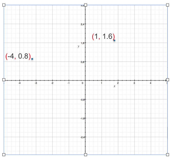
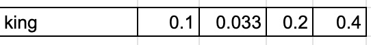
We can only visualize 3 dimensions, anything more than that you can just say it not visualize. Below is an example of 4 dimension vector representation of the word king
What is a Vector Database?
A Vector Database (VectorDB) is a specialized database system designed to store, manage, and efficiently query high-dimensional vector data. Unlike traditional relational databases that work with structured data in tables, VectorDBs are optimized for handling vector embeddings – numerical representations of data in multi-dimensional space.
In a VectorDB:
- Each item (like a document, image, or concept) is represented as a vector – a list of numbers that describe the item’s features or characteristics.
- These vectors are stored in a way that allows for fast similarity searches and comparisons.
- The database is optimized for operations like finding the nearest neighbors to a given vector, which is crucial for many AI and machine learning applications.
VectorDBs are particularly useful in scenarios where you need to find similarities or relationships between large amounts of complex data, such as in recommendation systems, image recognition, or natural language processing tasks.
Key Concepts
-
Vector Embeddings
- Vector embeddings are numerical representations of data in a multi-dimensional space.
- They capture semantic meaning and relationships between different pieces of information.
- In natural language processing, word embeddings are a common type of vector embedding. Each word is represented by a vector of real numbers, where words with similar meanings are closer in the vector space.
- For detail concepts of embedding please refer to earlier blog Embeddings
Let’s look at an example of Word Vector output generated by Word2Vec
from gensim.models import Word2Vec

# Example corpus (a list of sentences, where each sentence is a list of words)
sentences = [
    ["machine", "learning", "is", "fascinating"],
    ["gensim", "is", "a", "useful", "library", "for", "word", "embeddings"],
    ["vector", "representations", "are", "important", "for", "NLP", "tasks"]
]

# Train a Word2Vec model with 300-dimensional vectors
model = Word2Vec(sentences, vector_size=300, window=5, min_count=1, workers=4)

# Get the 300-dimensional vector for a specific word
word_vector = model.wv['machine']

# Print the vector
print(f"Vector for 'machine': {word_vector}")
Sample Output for 300 dimension vector
Vector for 'machine': [ 2.41737941e-03 -1.42750892e-03 -4.85344668e-03  3.12493594e-03, 4.84531874e-03 -1.00165956e-03  3.41092921e-03 -3.41384278e-03, 4.22888929e-03  1.44586214e-03 -1.35438916e-03 -3.27448458e-03
  4.70721726e-03 -4.50850562e-03  2.64214014e-03 -3.29884756e-03, -3.13906092e-03  1.09677911e-03 -4.94637461e-03  3.32896863e-03,2.03538216e-03 -1.52456785e-03  2.28793684e-03 -1.43519988e-03, 4.34566711e-03 -1.94705374e-03  1.93231280e-03  4.34081139e-03
  ...
  3.40303702e-03  1.58637420e-03 -3.31261402e-03  2.01543484e-03,4.39879852e-03  2.54576413e-03 -3.30528596e-03  3.01509819e-03,2.15555660e-03  1.64605413e-03  3.02376228e-03 -2.62048110e-03
  3.80181967e-03 -3.14147812e-03  2.23554621e-03  2.68812295e-03,1.80951719e-03  1.74256027e-03 -2.47024545e-03  4.06702763e-03,2.30203426e-03 -4.75471295e-03 -3.66776927e-03  2.06539119e-03]
- High Dimensional Space
- Vector databases typically work with vectors that have hundreds or thousands of dimensions. This high dimensionality allows for rich and nuanced representations of data.
- For example:
- A word might be represented by 300 dimensions
- An image could be represented by 1000 dimensions
- A user’s preferences might be captured in 500 dimensions
Why do you need a Vector Database when there is RDBMS like PostGreSQL or NoSQL DB like Elastic Search or MongoDB?
RDBMS
RDBMS are designed to store and manage structured data in a tabular format. They are based on the relational model, which defines data as a collection of tables, where each table represents a relation.
Key components of RDBMS:
- Tables: A collection of rows and columns, where each row represents a record and each column represents an attribute.
- Rows: Also known as records, they represent instances of an entity.
- Columns: Also known as attributes, they define the properties of an entity.
- Primary key: A unique identifier for each row in a table.
- Foreign key: A column in one table that references the primary key of another table, establishing a relationship between the two tables.
- Normalization: A process of organizing data into tables to minimize redundancy and improve data integrity.
Why RDBMS don’t apply to storing vectors:
- Data Representation:
- RDBMS store data in a tabular format, where each row represents an instance of an entity and each column represents an attribute.
- Vectors are represented as a sequence of numbers, which doesn’t fit well into the tabular structure of RDBMS.
- Query Patterns:
- RDBMS are optimized for queries based on joining tables and filtering data based on specific conditions.
- Vector databases are optimized for similarity search, which involves finding vectors that are closest to a given query vector. This type of query doesn’t align well with the traditional join-based queries of RDBMS.
- Data Relationships:
- RDBMS define relationships between entities using foreign keys and primary keys.
- In vector databases, relationships are implicitly defined by the proximity of vectors in the vector space. There’s no explicit need for foreign keys or primary keys.
- Performance Considerations:
- RDBMS are often optimized for join operations and range queries.
- Vector databases are optimized for similarity search, which requires efficient indexing and partitioning techniques.
Let’s also look at a table for a comparison of features
| Feature | VectorDB | RDBMS |
|---|---|---|
| Dimensional Efficiency | Designed to handle high-dimensional data efficiently | Performance degrades rapidly as dimensions increase |
| Similarity Search | Implement specialized algorithms for fast approximate nearest neighbor (ANN) searches | Lack native support for ANN algorithms, making similarity searches slow and computationally expensive |
| Indexing for Vector Spaces | Use index structures optimized for vector data (e.g., HNSW, IVF) | Rely on B-trees and hash indexes, which become ineffective in high-dimensional spaces |
| Vector Operations | Provide built-in, optimized support for vector operations | Require complex, often inefficient SQL queries to perform vector computations |
| Scalability for Vector Data | Designed to distribute vector data and parallelize similarity searches across multiple nodes efficiently | While scalable for traditional data, they’re not optimized for distributing and querying vector data at scale |
| Real-time Processing | Optimized for fast insertions and queries of vector data, supporting real-time applications | May struggle with the speed requirements of real-time vector processing, especially at scale |
| Storage Efficiency | Use compact, specialized formats for storing dense vector data | Less efficient when storing high-dimensional vectors, often requiring more space and slower retrieval |
| Machine Learning Integration | Seamlessly integrate with ML workflows, supporting operations common in AI applications | Require additional processing and transformations to work effectively with ML pipelines |
| Approximate Query Support | Often support approximate queries, trading off some accuracy for significant speed improvements | Primarily designed for exact queries, lacking native support for approximate vector searches |
In a nutshell, RDBMS are well-suited for storing and managing structured data, but they are not optimized for storing and querying vectors. Vector databases, on the other hand, are specifically designed for handling vectors and performing similarity search operations.
NoSQL Databases
NoSQL databases are designed to handle large datasets and unstructured or semi-structured data that don’t fit well into the relational model. They offer flexibility in data structures, scalability, and high performance.
Common types of NoSQL databases include:
- Key-value stores: Store data as key-value pairs.
- Document stores: Store data as documents, often in JSON or BSON format.
- Wide-column stores: Store data in wide columns, where each column can have multiple values.
- Graph databases: Store data as nodes and relationships, representing connected data.
Key characteristics of NoSQL databases:
- Flexibility: NoSQL databases offer flexibility in data structures, allowing for dynamic schema changes and accommodating evolving data requirements.
- Scalability: Many NoSQL databases are designed to scale horizontally, allowing for better performance and scalability as data volumes grow.
- High performance: NoSQL databases often provide high performance, especially for certain types of workloads.
- Eventual consistency: Some NoSQL databases prioritize availability and performance over strong consistency, offering eventual consistency guarantees.
Why NoSQL Databases Might Not Be Ideal for Storing and Retrieving Vectors
While NoSQL databases offer many advantages, they might not be the best choice for storing and retrieving vectors due to the following reasons:
- Data Representation: NoSQL databases, while flexible, might not be specifically optimized for storing and querying high-dimensional vectors. The data structures used in NoSQL databases might not be the most efficient for vector-based operations.
- Query Patterns: NoSQL databases are often designed for different query patterns than vector-based operations. While they can handle complex queries, they might not be as efficient for similarity search, which is a core operation for vector databases.
- Performance Considerations:
- Indexing: NoSQL databases often use different indexing techniques than RDBMS. While they can be efficient for certain types of queries, they might not be as optimized for vector-based similarity search.
- Memory requirements: For vector-based operations, especially in large-scale applications, the memory requirements can be significant. NoSQL databases like Elasticsearch, which are often used for full-text search and analytics, might require substantial memory resources to handle large vector datasets efficiently.
Elasticsearch as an Example:
Elasticsearch is a popular NoSQL database often used for full-text search and analytics. While it can be used to store and retrieve vectors, there are some considerations:
- Memory requirements: Storing and indexing large vector datasets in Elasticsearch can be memory-intensive, especially for high-dimensional vectors.
- Query performance: The performance of vector-based queries in Elasticsearch can depend on factors like the number of dimensions, the size of the dataset, and the indexing strategy used.
- Specialized plugins: Elasticsearch offers plugins like the
knnplugin that can be used to optimize vector-based similarity search. However, these plugins might have additional performance and memory implications.
In a nutshell, while NoSQL databases offer many advantages, their suitability for storing and retrieving vectors depends on specific use cases and requirements. For applications that heavily rely on vector-based similarity search and require high performance, specialized vector databases might be a more appropriate choice.
A Deeper Dive into Similarity Search in Vector Databases
Similarity search is a fundamental operation in vector databases, involving finding the closest matches to a given query vector from a large dataset of vectors. This is crucial for applications like recommendation systems, image search, and natural language processing.
Similarity measures, algorithms, and data structures are crucial for efficient similarity search. Similarity measures (e.g., cosine, Euclidean) quantify the closeness between vectors. Algorithms (e.g., brute force, LSH, HNSW) determine how vectors are compared and retrieved. Data structures (e.g., inverted indexes, hierarchical graphs) optimize storage and retrieval. The choice of these components depends on factors like dataset size, dimensionality, and desired accuracy. By selecting appropriate measures, algorithms, and data structures, you can achieve efficient and accurate similarity search in various applications. Let’s look in details about the different similarity measures and algorithms/datastructures in the below section.
Understanding Similarity Measures
- Cosine Similarity: Measures the angle between two vectors. It’s suitable when the magnitude of the vectors doesn’t matter (e.g., document similarity based on word counts).
import numpy as np

def cosine_similarity(v1, v2):
    """Calculates the cosine similarity between two vectors.

    Args:
        v1: The first vector.
        v2: The second vector.

    Returns:
        The cosine similarity between the two vectors.
    """

    dot_product = np.dot(v1, v2)
    norm_v1 = np.linalg.norm(v1)
    norm_v2 = np.linalg.norm(v2)

    return dot_product / (norm_v1 * norm_v2)

# Example usage
vector1 = np.array([1, 2, 3])
vector2 = np.array([4, 5, 6])
similarity = cosine_similarity(vector1, vector2)
print(similarity)
- Euclidean Distance: Measures the straight-line distance between two points in Euclidean space. It’s suitable when the magnitude of the vectors is important (e.g., image similarity based on pixel values).
import numpy as np

def euclidean_distance(v1, v2):
    """Calculates the Euclidean distance between two vectors.

    Args:
        v1: The first vector.
        v2: The second vector.

    Returns:
        The Euclidean distance between the two vectors.
    """

    return np.linalg.norm(v1 - v2)

# Example usage
vector1 = np.array([1, 2, 3])
vector2 = np.array([4, 5, 6])
distance = euclidean_distance(vector1, vector2)
print(distance)
- Hamming Distance: Measures the number of positions where two binary vectors differ. It’s useful for comparing binary data.
import numpy as np

def hamming_distance(v1, v2):
    """Calculates the Hamming distance between two binary vectors.

    Args:
        v1: The first binary vector.
        v2: The second binary vector.

    Returns:
        The Hamming distance between the two vectors.
    """

    return np.sum(v1 != v2)

# Example usage
vector1 = np.array([0, 1, 1, 0])
vector2 = np.array([1, 1, 0, 1])
distance = hamming_distance(vector1, vector2)
print(distance)
- Manhattan Distance: Also known as L1 distance, it measures the sum of absolute differences between corresponding elements of two vectors.
import numpy as np

def manhattan_distance(v1, v2):
    """Calculates the Manhattan distance between two vectors.

    Args:
        v1: The first vector.
        v2: The second vector.

    Returns:
        The Manhattan distance between the two vectors.
    """

    return np.sum(np.abs(v1 - v2))

# Example usage
vector1 = np.array([1, 2, 3])
vector2 = np.array([4, 5, 6])
distance = manhattan_distance(vector1, vector2)
print(distance)
Algorithms and Data Structures
Brute Force: is a straightforward but computationally expensive algorithm for finding the nearest neighbors in a dataset. It involves comparing the query vector with every other vector in the dataset to find the closest matches.
How Brute Force Works
- Iterate through the dataset: For each vector in the dataset, calculate its distance to the query vector.
- Maintain a list of closest neighbors: Keep track of the closest vectors found so far.
- Update the list: If the distance between the current vector and the query vector is smaller than the distance to the farthest neighbor in the list, replace the farthest neighbor with the current vector.
- Repeat: Continue this process until all vectors in the dataset have been compared.
Advantages and Disadvantages
- Advantages:
- Simple to implement.
- Guaranteed to find the exact nearest neighbors.
- Disadvantages:
- Extremely slow for large datasets.
- Inefficient for high-dimensional data.
Python Code Example
import numpy as np

def brute_force_search(query_vector, vectors, k=10):
    """Performs brute force search for the nearest neighbors.

    Args:
        query_vector: The query vector.
        vectors: The dataset of vectors.
        k: The number of nearest neighbors to find.

    Returns:
        A list of indices of the nearest neighbors.
    """

    distances = np.linalg.norm(vectors - query_vector, axis=1)
    nearest_neighbors = np.argsort(distances)[:k]
    return nearest_neighbors

# Example usage
query_vector = np.random.rand(128)
vectors = np.random.rand(1000, 128)
nearest_neighbors = brute_force_search(query_vector, vectors, k=10)
Brute Force is generally not suitable for large datasets or high-dimensional data due to its computational complexity. For these scenarios, more efficient algorithms like LSH, HNSW, or IVF-Flat are typically used. However, it can be useful for small datasets or as a baseline for comparison with other algorithms.
Locality Sensitive Hashing (LSH): is a technique used to efficiently find similar items in large datasets. It works by partitioning the vector space into buckets and hashing similar vectors into the same bucket. This makes it possible to quickly find approximate nearest neighbors without having to compare every vector in the dataset.
How LSH Works
- Hash Function Selection: Choose a hash function that is sensitive to the distance between vectors. This means that similar vectors are more likely to be hashed into the same bucket.
- Hash Table Creation: Create multiple hash tables, each using a different hash function.
- Vector Hashing: For each vector, hash it into each hash table.
- Query Processing: When a query vector is given, hash it into each hash table.
- Candidate Selection: Retrieve all vectors that are in the same buckets as the query vector.
- Similarity Calculation: Calculate the actual similarity between the query vector and the candidate vectors.
LSH Families
- Random Projection: Projects vectors onto random hyperplanes.
- MinHash: Used for comparing sets of items.
- SimHash: Used for comparing documents based on their shingles.
LSH Advantages and Disadvantages
- Advantages:
- Efficient for large datasets.
- Can be used for approximate nearest neighbor search.
- Can be parallelized.
- Disadvantages:
- Can introduce false positives or negatives.
- Accuracy can be affected by the choice of hash functions and the number of hash tables.
Python Code Example using Annoy
from annoy import Annoy

# Create an Annoy index with LSH
annoy_index = Annoy(128, metric='angular', n_trees=10)

# Add vectors to the index
for i in range(1000):
    vector = np.random.rand(128)
    annoy_index.add_item(i, vector)

# Build the index
annoy_index.build()

# Search for nearest neighbors
query_vector = np.random.rand(128)
nns = annoy_index.get_nns_by_vector(query_vector, 10)
Note: The n_trees parameter in Annoy determines the number of hash tables used. A larger number of trees generally improves accuracy but can increase memory usage.
By understanding the fundamentals of LSH and carefully selecting the appropriate parameters, you can effectively use it for similarity search in your applications.
Hierarchical Navigable Small World (HNSW): is a highly efficient algorithm for approximate nearest neighbor search in high-dimensional spaces. It constructs a hierarchical graph structure that allows for fast and accurate retrieval of similar items.
How HNSW Works
- Initialization: The algorithm starts by creating a single layer with all data points.
- Layer Creation: New layers are added iteratively. Each new point is connected to a subset of existing points based on their distance.
- Hierarchical Structure: The layers form a hierarchical structure, with higher layers having fewer connections and lower layers having more connections.
- Search: To find the nearest neighbors of a query point, the search starts from the top layer and gradually moves down the hierarchy, following the connections to find the most promising candidates.
Advantages of HNSW
- High Accuracy: HNSW often achieves high accuracy, even for high-dimensional data.
- Efficiency: It is very efficient for large datasets and can handle dynamic updates.
- Flexibility: The algorithm can be adapted to different distance metrics and data distributions.
Python Code Example using NMSLIB
from nmslib import NMSLIB

# Create an HNSW index
nmslib_index = NMSLIB.init(method='hnsw', space='cos')

# Add vectors to the index
nmslib_index.addDataPointBatch(vectors)

# Create the index
nmslib_index.createIndex()

# Search for nearest neighbors
query_vector = np.random.rand(128)
knn = nmslib_index.knnQuery(query_vector, k=10)
Note: The space parameter in NMSLIB specifies the distance metric used (e.g., cos for cosine similarity). You can also customize other parameters like the number of layers and the number of connections per layer to optimize performance for your specific application.
HNSW is a powerful algorithm for approximate nearest neighbor search, offering a good balance between accuracy and efficiency. It’s particularly well-suited for high-dimensional data and can be used in various applications, such as recommendation systems, image search, and natural language processing.
IVF-Flat: is a hybrid indexing technique that combines Inverted File (IVF) and Flat Hierarchical Indexing (Flat) to efficiently perform approximate nearest neighbor search (ANN) in high-dimensional vector spaces. It’s particularly effective for large datasets and high-dimensional vectors.
How IVF-Flat Works
- Quantization: The dataset is divided into
nquantized subspaces (quantization cells). Each vector is assigned to a cell based on its similarity to a representative point (centroid) of the cell. - Inverted File: An inverted index is created, where each quantized cell is associated with a list of vectors belonging to that cell.
- Flat Index: For each quantized cell, a flat index (e.g., a linear scan or a tree-based structure) is built to store the vectors assigned to that cell.
- Query Processing: When a query vector is given, it’s first quantized to find the corresponding cell. Then, the flat index for that cell is searched for the nearest neighbors.
- Refinement: The top candidates from the flat index can be further refined using exact nearest neighbor search or other techniques to improve accuracy.
Advantages of IVF-Flat
- Efficiency: IVF-Flat can be significantly faster than brute-force search for large datasets.
- Accuracy: It can achieve good accuracy, especially when combined with refinement techniques.
- Scalability: It can handle large datasets and high-dimensional vectors.
- Flexibility: The number of quantized cells and the type of flat index can be adjusted to balance accuracy and efficiency.
Python Code Example using Faiss
import faiss

# Create an IVF-Flat index
index = faiss.IndexIVFFlat(faiss.IndexFlatL2(dim), nlist, nprobe)

# Add vectors to the index
index.add(vectors)

# Search for nearest neighbors
query_vector = np.random.rand(dim)
distances, indices = index.search(query_vector, k)
In this example:
dimis the dimensionality of the vectors.nlistis the number of quantized cells.nprobeis the number of cells to query during search.
IVF-Flat is a powerful technique for approximate nearest neighbor search in vector databases, offering a good balance between efficiency and accuracy. By carefully tuning the parameters, you can optimize its performance for your specific application.
ScanNN: is a scalable and efficient approximate nearest neighbor search algorithm designed for large-scale datasets. It combines inverted indexes with quantization techniques to achieve high performance.
How ScanNN Works
- Quantization: The dataset is divided into quantized subspaces (quantization cells). Each vector is assigned to a cell based on its similarity to a representative point (centroid) of the cell.
- Inverted Index: An inverted index is created, where each quantized cell is associated with a list of vectors belonging to that cell.
- Scan: During query processing, the query vector is quantized to find the corresponding cell. Then, the vectors in that cell are scanned to find the nearest neighbors.
- Refinement: The top candidates from the scan can be further refined using exact nearest neighbor search or other techniques to improve accuracy.
Advantages of ScanNN
- Scalability: ScanNN can handle large datasets and high-dimensional vectors efficiently.
- Efficiency: It uses inverted indexes to reduce the search space, making it faster than brute-force search.
- Accuracy: ScanNN can achieve good accuracy, especially when combined with refinement techniques.
- Flexibility: The number of quantized cells and the refinement strategy can be adjusted to balance accuracy and efficiency.
Python Code Example using Faiss
import faiss

# Create a ScanNN index
index = faiss.IndexScanNN(faiss.IndexFlatL2(dim), nlist, nprobe)

# Add vectors to the index
index.add(vectors)

# Search for nearest neighbors
query_vector = np.random.rand(dim)
distances, indices = index.search(query_vector, k)
In this example:
dimis the dimensionality of the vectors.nlistis the number of quantized cells.nprobeis the number of cells to query during search.
ScanNN is a powerful algorithm for approximate nearest neighbor search in large-scale applications. It offers a good balance between efficiency and accuracy, making it a popular choice for various tasks, such as recommendation systems, image search, and natural language processing.
Disk-ANN: is a scalable approximate nearest neighbor search algorithm designed for very large datasets that don’t fit entirely in memory. It combines inverted files with on-disk storage to efficiently handle large-scale vector search.
How Disk-ANN Works
- Quantization: The dataset is divided into quantized subspaces (quantization cells), similar to IVF-Flat.
- Inverted Index: An inverted index is created, where each quantized cell is associated with a list of vectors belonging to that cell.
- On-Disk Storage: The inverted index and the vectors themselves are stored on disk, allowing for efficient handling of large datasets.
- Query Processing: When a query vector is given, it’s quantized to find the corresponding cell. The inverted index is used to retrieve the vectors in that cell from disk.
- Refinement: The retrieved vectors can be further refined using exact nearest neighbor search or other techniques to improve accuracy.
Advantages of Disk-ANN
- Scalability: Disk-ANN can handle extremely large datasets that don’t fit in memory.
- Efficiency: It uses inverted indexes and on-disk storage to optimize performance for large-scale search.
- Accuracy: Disk-ANN can achieve good accuracy, especially when combined with refinement techniques.
- Flexibility: The number of quantized cells and the refinement strategy can be adjusted to balance accuracy and efficiency.
Python Code Example using Faiss
import faiss

# Create a Disk-ANN index
index = faiss.IndexDiskANN(faiss.IndexFlatL2(dim), filename, nlist, nprobe)

# Add vectors to the index
index.add(vectors)

# Search for nearest neighbors
query_vector = np.random.rand(dim)
distances, indices = index.search(query_vector, k)
In this example:
filenameis the path to the disk file where the index will be stored.- Other parameters are the same as in IVF-Flat.
Disk-ANN is a powerful algorithm for approximate nearest neighbor search in very large datasets. It provides a scalable and efficient solution for handling massive amounts of data while maintaining good accuracy.
Vector Database Comparison: Features, Use Cases, and Selection Guide
Just like in RDBMS or NOSQL world there are lot of choices for different databases, Vector Databases also have quite a bit choices, choosing the right one for your application matters quite a bit. Below table compares key features, use-cases and a selection guide
| VectorDB | Key Features | Best For | When to Choose |
|---|---|---|---|
| Pinecone | Fully managed service, Real-time updates, Hybrid search (vector + metadata), Serverless | Production-ready applications, Rapid development, Scalable solutions | When you need a fully managed solution, For applications requiring real-time updates, When combining vector search with metadata filtering |
| Milvus | Open-source, Scalable to billions of vectors, Supports multiple index types, Hybrid search capabilities | Large-scale vector search, On-premises deployments, Customizable solutions | When you need an open-source solution, for very large-scale vector search applications, When you require fine-grained control over indexing |
| Qdrant | Open-source, Rust-based for high performance, Supports filtering with payload, On-prem and cloud options | High-performance vector search, Applications with complex filtering needs | When performance is critical, for applications requiring advanced filtering, When you need both cloud and on-prem options |
| Weaviate | Open-source, GraphQL API, Multi-modal data support, AI-first database | Semantic search applications, Multi-modal data storage and retrieval | When working with multiple data types (text, images, etc.), If you prefer GraphQL for querying, for AI-centric applications |
| Faiss (Facebook AI Similarity Search) | Open-source, Highly efficient for dense vectors, GPU support | Research and experimentation, Large-scale similarity search | When you need low-level control, for integration into custom systems, When GPU acceleration is beneficial |
| Elasticsearch with vector search | Full-text search + vector capabilities, Mature ecosystem and extensive analytics features | Applications combining traditional search and vector search | when you need rich text analytics, When you’re already using Elasticsearch, For hybrid search applications (text + vector), When you need advanced analytics alongside vector search |
| pgvector (PostgreSQL extension) | Vector similarity search in PostgreSQL, Integrates with existing PostgreSQL databases | Adding vector capabilities to existing PostgreSQL systems, Small to medium-scale applications | When you’re already heavily invested in PostgreSQL, for projects that don’t require specialized vector DB features, When simplicity and familiarity are priorities |
| Vespa | Open-source, Combines full-text search, vector search, and structured data, Real-time indexing and serving | Complex search and recommendation systems, Applications requiring structured, text, and vector data | For large-scale, multi-modal search applications, When you need a unified platform for different data types, For real-time, high-volume applications |
| AWS OpenSearch | Fully managed AWS service, Combines traditional full-text search capabilities with vector-based similarity search. | When you need to search for both text-based content and vectors. | When you need to perform real-time searches and analytics on large datasets. When you want to leverage the broader AWS ecosystem for your application. For applications that require processing billions of vectors. |
Conclusion
For my previous startup that I (Malaikannan Sankarasubbu) founded Datalog dot ai doing a low code virtual assistant platform, we heavily leveraged FAISS to do Intent similarity, from that point to now there are quite a few options for Vector Databases
Vector databases have emerged as a powerful tool for handling unstructured and semi-structured data, offering efficient similarity search capabilities and supporting a wide range of applications. By understanding the fundamentals of vector databases, including similarity measures, algorithms, and data structures, you can select the right approach for your specific needs.
In future blog posts, we will delve deeper into performance considerations, including indexing techniques, hardware optimization, and best practices for scaling vector databases. We will also explore real-world use cases and discuss the challenges and opportunities that lie ahead in the field of vector databases.