Embeddings

31 Jul 2024

Computers are meant to crunch numbers; it goes back to the original design of these machines. Representing text as numbers is the holy grail of Natural Language Processing (NLP), but how do we do that? Over the years, various techniques have been developed to achieve this. Early methods like n-grams (like bigrams and trigrams) and TF-IDF were able to convert words into numbers. Not just one number, a collection of them. Each word is represented by the collection of numbers. The collection of numbers is called vector and it had a size that is fixed called the dimension of the vector. Though they were useful, they had their limitations. The most important of the limitations is that the vectors for each words stands alone, i.e we could not do any mathematical operations like addition or subtraction between the vectors(actually we could but the resulting vector will not represent any word). That is where embeddings come in. Embedding is also a vector, and so each word get a corresponding vector but we can now do King - Man + Woman that will give us a vector which is close to the vector corresponding to Queen. Why is this useful? That is what we are going to explore in this article.

What are Embeddings?

Embeddings are numerical representations of text data where words or phrases from the vocabulary are mapped to vectors of real numbers. This mapping is crucial because it allows us to quantify and manipulate textual data in a way that machines can understand and process.

We understand what a word is, lets see what a vector is. A vector is a sequence of numbers that forms a group. For example

• (3) is a one dimensional vector.
• (2,8) is a two dimensional vector.
• (12,6,7,4) is a four dimensional vector.

A vector can be represented as by plotting on a graph. Lets take a 2D example

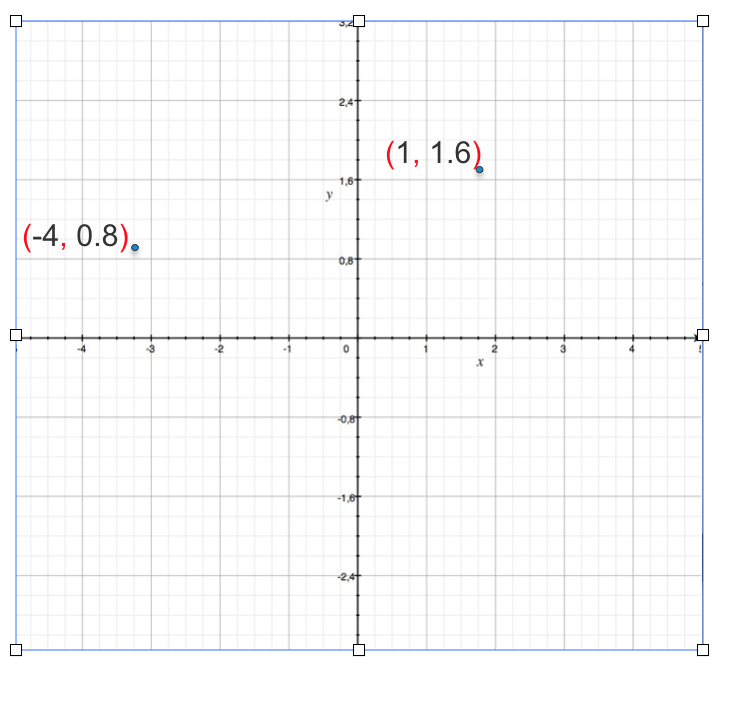
We can only 3 dimensions, anything more than that you can just say it not visualize.

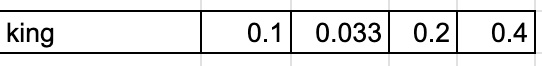
Below is an example of 4 dimension vector representation of the word king

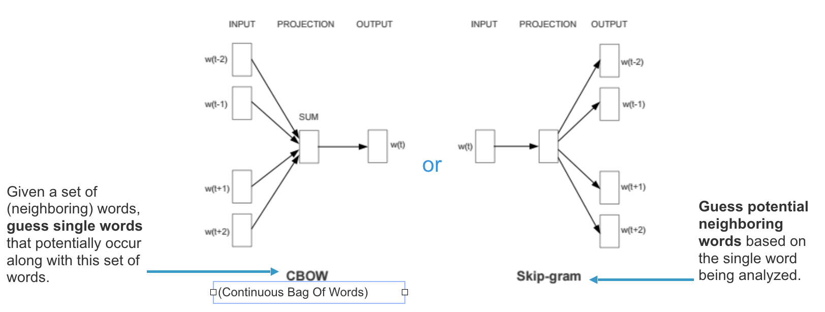
One of the seminal papers that have come out from Google is Word2vec. Lets see how Word2Vec works to get a conceptual understanding of how embedding works

How Word2Vec works

For a input text it looks at each word and the context of words around it. It trains on the text, and recognizes the order of each word, and the structure of the sentences. At the end of training each word is represented by a vector of N (mostly in 100 to 300 range) dimension.

When we train word2vec algorithm in the example discussed above “SanFrancisco is a beautiful California city. LosAngeles is a lovely California metropolis”

Lets assume that it outputs 2 dimension vectors for each words, since we can’t visualize anything more than 3 dimension.

• SanFrancisco (6,6)
• beautiful (-13,-4)
• California (10,8)
• city (2,10)
• LosAngeles (6.5,5)
• lovely(-12,-7)
• metropolis(2.5,8)

Below is a 2D Plot of vectors

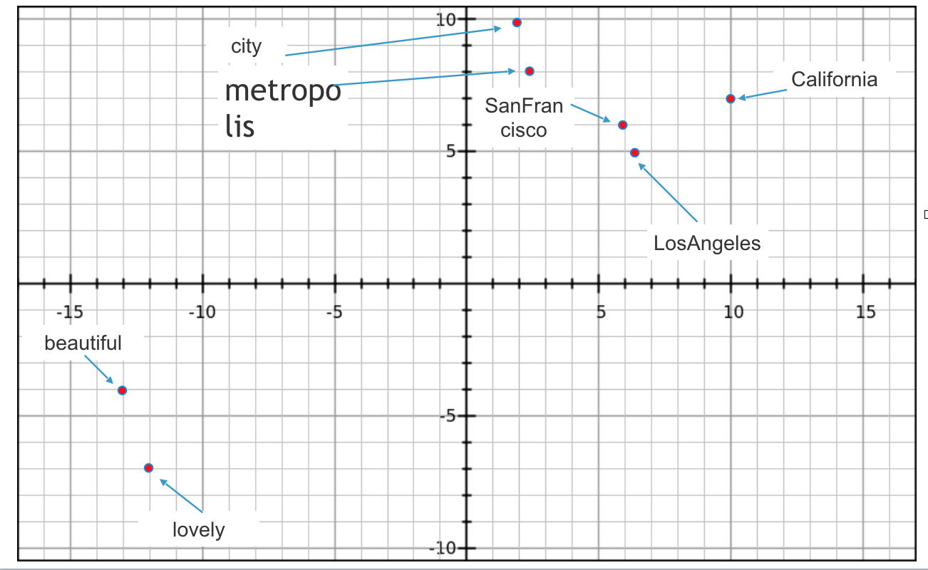
You can see in the image that Word2vec algorithm inferred from the input text. SanFrancisco and LosAngeles are grouped together. Beautiful and lovely are grouped together. City and metropolis are grouped together. Beauty about this is, Word2vec deduced this purely from data, without being explicitly taught english or geography.

You will see more embedding approaches in the below sections

Key Characteristics of Embeddings:

1. Dimensionality: Embeddings are vectors of fixed size. Common sizes range from 50 to 300 dimensions, though they can be larger depending on the complexity of the task.
2. Continuous Space: Unlike traditional one-hot encoding, embeddings are dense and reside in a continuous vector space, making them more efficient and informative.
3. Semantic Proximity: Words with similar meanings tend to have vectors that are close to each other in the embedding space.

The Evolution of Embeddings

Embeddings have evolved significantly over the years. Here are some key milestones:

1. Word2Vec (2013): Developed by Mikolov et al. at Google, Word2Vec was one of the first algorithms to create word embeddings. It uses two architectures—Continuous Bag of Words (CBOW) and Skip-gram—to learn word associations.

2. GloVe (2014): Developed by the Stanford NLP Group, GloVe (Global Vectors for Word Representation) improves upon Word2Vec by incorporating global statistical information of the corpus.

3. FastText (2016): Developed by Facebook’s AI Research (FAIR) lab, FastText extends Word2Vec by considering subword information, which helps in handling out-of-vocabulary words and capturing morphological details.

4. ELMo (2018): Developed by the Allen Institute for AI, ELMo (Embeddings from Language Models) generates context-sensitive embeddings, meaning the representation of a word changes based on its context in a sentence.

5. BERT (2018): Developed by Google, BERT (Bidirectional Encoder Representations from Transformers) revolutionized embeddings by using transformers to understand the context of a word bidirectionally. This model significantly improved performance on various NLP tasks.

From Word Embeddings to Sentence Embeddings

While word embeddings provide a way to represent individual words, they do not capture the meaning of entire sentences or documents. This limitation led to the development of sentence embeddings, which are designed to represent longer text sequences.

Word Embeddings

Word embeddings, such as those created by Word2Vec, GloVe, and FastText, map individual words to vectors. These embeddings capture semantic similarities between words based on their context within a large corpus of text. For example, the words “king” and “queen” might be close together in the embedding space because they often appear in similar contexts.

Sentence Embeddings

Sentence embeddings extend the concept of word embeddings to entire sentences or even paragraphs. These embeddings aim to capture the meaning of a whole sentence, taking into account the context and relationships between words within the sentence. There are several methods to create sentence embeddings:

1. Averaging Word Embeddings: One of the simplest methods is to average the word embeddings of all words in a sentence. While this method is straightforward, it often fails to capture the nuances and syntactic structures of sentences.

2. Doc2Vec: Developed by Mikolov and Le, Doc2Vec extends Word2Vec to larger text segments by considering the paragraph as an additional feature during training. This method generates embeddings for sentences or documents that capture more context compared to averaging word embeddings.

3. Recurrent Neural Networks (RNNs): RNNs, particularly Long Short-Term Memory (LSTM) networks, can be used to generate sentence embeddings by processing the sequence of words in a sentence. The hidden state of the RNN after processing the entire sentence can serve as the sentence embedding.

4. Transformers (BERT, GPT, etc.): Modern approaches like BERT and GPT use transformer architectures to generate context-aware embeddings for sentences. These models can process a sentence bidirectionally, capturing dependencies and relationships between words more effectively than previous methods.

Example: BERT Sentence Embeddings

BERT (Bidirectional Encoder Representations from Transformers) has set a new standard for generating high-quality sentence embeddings. By processing a sentence in both directions, BERT captures the full context of each word in relation to the entire sentence. The embeddings generated by BERT can be fine-tuned for various NLP tasks, such as sentiment analysis, question answering, and text classification.

To create a sentence embedding with BERT, you can use the hidden states of the transformer model. Typically, the hidden state corresponding to the [CLS] token (which stands for “classification”) is used as the sentence embedding.

How to Generate Embeddings

Generating embeddings involves training a model on a large corpus of text data. Here’s a step-by-step guide to generating word and sentence embeddings:

Generating Word Embeddings with Word2Vec

1. Data Preparation: Collect and preprocess a large text corpus. This involves tokenizing the text, removing stop words, and handling punctuation.

2. Training the Model: Use the Word2Vec algorithm to train the model. You can choose between the CBOW or Skip-gram architecture. Libraries like Gensim in Python provide easy-to-use implementations of Word2Vec.

   from gensim.models import Word2Vec
   
   # Example sentences
   sentences = [["I", "love", "machine", "learning"], ["Word2Vec", "is", "great"]]
   
   # Train Word2Vec model
   model = Word2Vec(sentences, vector_size=100, window=5, min_count=1, workers=4)
   

3. Using the Embeddings: Once the model is trained, you can use it to get the embedding for any word in the vocabulary.

   word_embedding = model.wv['machine']
   

Generating Sentence Embeddings with BERT

1. Install Transformers Library: Use the Hugging Face Transformers library to easily work with BERT.

   pip install transformers
   

2. Load Pretrained BERT Model: Load a pretrained BERT model and tokenizer.

   from transformers import BertTokenizer, BertModel
   import torch
   
   tokenizer = BertTokenizer.from_pretrained('bert-base-uncased')
   model = BertModel.from_pretrained('bert-base-uncased')
   

3. Tokenize Input Text: Tokenize your input text and convert it to input IDs and attention masks.

   sentence = "BERT is amazing for sentence embeddings."
   inputs = tokenizer(sentence, return_tensors='pt')
   

4. Generate Embeddings: Pass the inputs through the BERT model to get the embeddings.

   with torch.no_grad():
       outputs = model(**inputs)
   
   # The [CLS] token embedding
   sentence_embedding = outputs.last_hidden_state[0][0]
   

5. Using the Embeddings: The sentence_embedding can now be used for various NLP tasks.

Data Needed for Training Embeddings

The quality of embeddings heavily depends on the data used for training. Here are key considerations regarding the data needed:

1. Size of the Corpus: A large corpus is generally required to capture the diverse contexts in which words can appear. For example, training Word2Vec or BERT models typically requires billions of words. The larger the corpus, the better the embeddings can capture semantic nuances.

2. Diversity of the Corpus: The corpus should cover a wide range of topics and genres to ensure that the embeddings are generalizable. This means including text from various domains such as news articles, books, social media, academic papers, and more.

3. Preprocessing: Proper preprocessing of the corpus is essential. This includes:
   • Tokenization: Splitting text into words or subwords.
   • Lowercasing: Converting all text to lowercase to reduce the vocabulary size.
   • Removing Punctuation and Stop Words: Cleaning the text by removing unnecessary punctuation and common stop words that do not contribute to the meaning.
   • Handling Special Characters: Dealing with special characters, numbers, and other non-alphabetic tokens appropriately.

4. Domain-Specific Data: For specialized applications, it is beneficial to include domain-specific data. For instance, medical embeddings should be trained on medical literature to capture the specialized vocabulary and context of the field.

5. Balanced Dataset: Ensuring that the dataset is balanced and not biased towards a particular topic or genre helps in creating more neutral and representative embeddings.

6. Data Augmentation: In cases where data is limited, data augmentation techniques such as back-translation, paraphrasing, and synthetic data generation can be used to enhance the corpus.

Applications of Sentence Embeddings

Sentence embeddings have a wide range of applications in NLP:

1. Text Classification: Sentence embeddings are used to represent sentences for classification tasks, such as identifying the topic of a sentence or determining the sentiment expressed in a review.
2. Semantic Search: By comparing sentence embeddings, search engines can retrieve documents that are semantically similar to a query, even if the exact keywords are not matched.
3. Summarization

: Sentence embeddings help in generating summaries by identifying the most important sentences in a document based on their semantic content.

1. Translation: Sentence embeddings improve machine translation systems by providing a richer representation of the source sentence, leading to more accurate translations.

Embedding Dimension Reduction Methods

High-dimensional embeddings can be computationally expensive and may contain redundant information. Dimension reduction techniques help in simplifying these embeddings while preserving their essential characteristics. Here are some common methods:

1. Principal Component Analysis (PCA): PCA is a linear method that reduces the dimensionality of data by transforming it into a new coordinate system where the greatest variances by any projection of the data come to lie on the first coordinates (principal components).

   from sklearn.decomposition import PCA
   
   # Assuming 'embeddings' is a numpy array of shape (n_samples, n_features)
   pca = PCA(n_components=50)
   reduced_embeddings = pca.fit_transform(embeddings)
   

2. t-Distributed Stochastic Neighbor Embedding (t-SNE): t-SNE is a nonlinear technique primarily used for visualizing high-dimensional data by reducing it to two or three dimensions.

   from sklearn.manifold import TSNE
   
   tsne = TSNE(n_components=2)
   reduced_embeddings = tsne.fit_transform(embeddings)
   

3. Uniform Manifold Approximation and Projection (UMAP): UMAP is another nonlinear technique that is faster and often more effective than t-SNE for dimension reduction, especially for larger datasets.

   import umap
   
   reducer = umap.UMAP(n_components=2)
   reduced_embeddings = reducer.fit_transform(embeddings)
   

4. Autoencoders: Autoencoders are a type of neural network used to learn efficient codings of input data. An autoencoder consists of an encoder and a decoder. The encoder compresses the input into a lower-dimensional latent space, and the decoder reconstructs the input from this latent space.

   from tensorflow.keras.layers import Input, Dense
   from tensorflow.keras.models import Model
   
   # Define encoder
   input_dim = embeddings.shape[1]
   encoding_dim = 50  # Size of the reduced dimension
   input_layer = Input(shape=(input_dim,))
   encoded = Dense(encoding_dim, activation='relu')(input_layer)
   
   # Define decoder
   decoded = Dense(input_dim, activation='sigmoid')(encoded)
   
   # Build the autoencoder model
   autoencoder = Model(input_layer, decoded)
   encoder = Model(input_layer, encoded)
   
   # Compile and train the autoencoder
   autoencoder.compile(optimizer='adam', loss='mean_squared_error')
   autoencoder.fit(embeddings, embeddings, epochs=50, batch_size=256, shuffle=True)
   
   # Get the reduced embeddings
   reduced_embeddings = encoder.predict(embeddings)
   

5. Random Projection: Random projection is a simple and computationally efficient technique to reduce dimensionality. It is based on the Johnson-Lindenstrauss lemma, which states that high-dimensional data can be embedded into a lower-dimensional space with minimal distortion.

   from sklearn.random_projection import SparseRandomProjection
   
   transformer = SparseRandomProjection(n_components=50)
   reduced_embeddings = transformer.fit_transform(embeddings)
   

Evaluating Embeddings

Evaluating embeddings is crucial to ensure that they capture meaningful relationships and semantics. Here are some common methods to evaluate embeddings:

1. Intrinsic Evaluation: These methods evaluate the quality of embeddings based on predefined linguistic tasks or properties without involving downstream tasks.

   • Word Similarity: Measure the cosine similarity between word pairs and compare with human-annotated similarity scores. Popular datasets include WordSim-353 and SimLex-999.

     from scipy.spatial.distance import cosine
     
     similarity = 1 - cosine(embedding1, embedding2)
     

   • Analogy Tasks: Evaluate embeddings based on their ability to solve word analogy tasks, such as “king - man + woman = queen.” Datasets like Google Analogy dataset are commonly used.

     def analogy(model, word1, word2, word3):
         vec = model[word1] - model[word2] + model[word3]
         return model.most_similar([vec])[0][0]
     

2. Extrinsic Evaluation: These methods evaluate embeddings based on their performance on downstream NLP tasks.

   • Text Classification: Use embeddings as features for text classification tasks and measure performance using metrics like accuracy, precision, recall, and F1 score.

     from sklearn.linear_model import LogisticRegression
     from sklearn.metrics import accuracy_score
     
     model = LogisticRegression()
     model.fit(train_embeddings, train_labels)
     predictions = model.predict(test_embeddings)
     accuracy = accuracy_score(test_labels, predictions)
     

   • Named Entity Recognition (NER): Evaluate embeddings by their performance on NER tasks, measuring precision, recall, and F1 score.

     # Example using spaCy for NER
     import spacy
     from spacy.tokens import DocBin
     
     nlp = spacy.load("en_core_web_sm")
     nlp.entity.add_label("ORG")
     
     train_docs = [nlp(text) for text in train_texts]
     train_db = DocBin(docs=train_docs)
     

   • Machine Translation: Assess the quality of embeddings by their impact on machine translation tasks, using BLEU or METEOR scores.

3. Clustering and Visualization: Visualizing embeddings using t-SNE or UMAP can provide qualitative insights into the structure and quality of embeddings.

   import matplotlib.pyplot as plt
   
   tsne = TSNE(n_components=2)
   reduced_embeddings = tsne.fit_transform(embeddings)
   
   plt.scatter(reduced_embeddings[:, 0], reduced_embeddings[:, 1])
   for i, word in enumerate(words):
       plt.annotate(word, xy=(reduced_embeddings[i, 0], reduced_embeddings[i, 1]))
   plt.show()
   

Similarity vs. Retrieval Embeddings

Embeddings can be tailored for different purposes, such as similarity or retrieval tasks. Understanding the distinction between these two types of embeddings is crucial for optimizing their use in various applications.

Similarity Embeddings

Similarity embeddings are designed to capture the semantic similarity between different pieces of text. The primary goal is to ensure that semantically similar texts have similar embeddings.

Use Cases:

• Semantic Search: Finding documents or sentences that are semantically similar to a query.
• Recommendation Systems: Recommending items (e.g., articles, products) that are similar to a given item.
• Paraphrase Detection: Identifying sentences or phrases that convey the same meaning.

Evaluation:

• Cosine Similarity: Measure the cosine similarity between embeddings to evaluate their closeness.

  from sklearn.metrics.pairwise import cosine_similarity
  
  similarity = cosine_similarity([embedding1], [embedding2])
  

• Clustering: Grouping similar items together using clustering algorithms like K-means.

  from sklearn.cluster import KMeans
  
  kmeans = KMeans(n_clusters=5)
  clusters = kmeans.fit_predict(embeddings)
  

Retrieval Embeddings

Retrieval embeddings are optimized for information retrieval tasks, where the goal is to retrieve the most relevant documents from a large corpus based on a query.

Use Cases:

• Search Engines: Retrieving relevant web pages or documents based on user queries.
• Question Answering Systems: Finding relevant passages or documents that contain the answer to a user’s question.
• Document Retrieval: Retrieving documents that are most relevant to a given query.

Evaluation:

• Precision and Recall: Measure the accuracy of retrieved documents using precision, recall, and F1 score.

  from sklearn.metrics import precision_score, recall_score, f1_score
  
  precision = precision_score(true_labels, predicted_labels, average='weighted')
  recall = recall_score(true_labels, predicted_labels, average='weighted')
  f1 = f1_score(true_labels, predicted_labels, average='weighted')
  

• Mean Reciprocal Rank (MRR): Evaluate the rank of the first relevant document.

  def mean_reciprocal_rank(rs):
      """Score is reciprocal of the rank of the first relevant item
      First element is 'rank 1'.  Relevance is binary (nonzero is relevant).
      Example from information retrieval with binary relevance:
      >>> rs = [[0, 0, 1], [0, 1, 0], [1, 0, 0]]
      >>> mean_reciprocal_rank(rs)
      0.61111111111111105
      """
      rs = (np.asarray(r).nonzero()[0] for r in rs)
      return np.mean([1. / (r[0] + 1) if r.size else 0. for r in rs])
  

Symmetric vs. Asymmetric Embeddings

Symmetric and asymmetric embeddings are designed to handle different types of relationships in data, and understanding their differences can help in choosing the right approach for specific tasks.

Symmetric Embeddings

Symmetric embeddings are used when the relationship between two items is mutual. The similarity between two items is expected to be the same regardless of the order in which they are compared.

Use Cases:

• Similarity Search: Comparing the similarity between two items, such as text or images, where the similarity score should be the same in both directions.
• Collaborative Filtering: Recommending items

based on mutual user-item interactions, where the relationship is bidirectional.

Evaluation:

• Cosine Similarity: Symmetric embeddings often use cosine similarity to measure the closeness of vectors.

  similarity = cosine_similarity([embedding1], [embedding2])
  

Asymmetric Embeddings

Asymmetric embeddings are used when the relationship between two items is directional. The similarity or relevance of one item to another may not be the same when the order is reversed.

Use Cases:

• Information Retrieval: Retrieving relevant documents for a query, where the relevance of a document to a query is not necessarily the same as the relevance of the query to the document.
• Knowledge Graph Embeddings: Representing entities and relationships in a knowledge graph, where the relationship is directional (e.g., parent-child, teacher-student).

Evaluation:

• Rank-Based Metrics: Asymmetric embeddings often use rank-based metrics like Mean Reciprocal Rank (MRR) and Normalized Discounted Cumulative Gain (NDCG) to evaluate performance.

  def mean_reciprocal_rank(rs):
      rs = (np.asarray(r).nonzero()[0] for r in rs)
      return np.mean([1. / (r[0] + 1) if r.size else 0. for r in rs])
  

The Future of Embeddings

The field of embeddings is rapidly evolving. Researchers are exploring new ways to create more efficient and accurate representations, such as using unsupervised learning and combining embeddings with other techniques like graph networks. The ongoing advancements in this area promise to further enhance the capabilities of NLP systems.

Conclusion

Embeddings have revolutionized the field of NLP, providing a robust and efficient way to represent and process textual data. From word embeddings to sentence embeddings, these techniques have enabled significant advancements in how machines understand and interact with human language. With the help of dimension reduction methods, evaluation techniques, and tailored similarity and retrieval embeddings, embeddings can be optimized for a wide range of NLP tasks. Understanding the differences between symmetric and asymmetric embeddings further allows for more specialized applications. As we continue to develop more sophisticated models and techniques, embeddings will undoubtedly play a crucial role in advancing our understanding and interaction with human language.